Markov chains and stationary distributions

Many processes evolve in steps where the next state depends only on the current one, not the full history: a random walk, a shuffled card deck, a token sequence under a simple model. A Markov chain captures this, and its long-run behavior is read off from the eigenstructure of a single matrix, tying probability back to linear algebra.

The Markov property

A sequence of random variables $X_0, X_1, X_2, \dots$ taking values in a finite state set is a Markov chain if the future depends on the past only through the present[1]:

This memorylessness is the defining assumption. The one-step dynamics are collected in the transition matrix $P$ with entries $P_{ij} = P(X_{t+1} = j \mid X_t = i)$. Each row sums to 1 (from state $i$ the chain must go somewhere), making $P$ a row-stochastic matrix.

Distributions evolve by matrix multiplication

Represent the distribution over states at time $t$ as a row vector $\pi^{(t)}$, with $\pi^{(t)}_i = P(X_t = i)$. One step forward uses the law of total probability:

which is the vector-matrix product $\pi^{(t+1)} = \pi^{(t)} P$. After $n$ steps,

The $n$-step transition probabilities are the entries of $P^n$. Evolving the chain is repeatedly multiplying by $P$.

Stationary distribution

A distribution $\pi$ is stationary if it is unchanged by a step[2]:

The equation $\pi P = \pi$ says $\pi$ is a left eigenvector of $P$ with eigenvalue 1. Every row-stochastic matrix has eigenvalue 1: the all-ones column vector $\mathbf{1}$ satisfies $P\mathbf{1} = \mathbf{1}$ (rows sum to 1), so 1 is an eigenvalue, and left and right eigenvalues coincide. All other eigenvalues have magnitude $\le 1$ (Gershgorin / Perron-Frobenius).

Convergence to stationarity

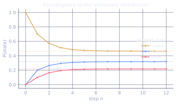
If the chain is irreducible (every state reachable from every other) and aperiodic (no forced cycles), the Perron-Frobenius theorem guarantees a unique stationary distribution $\pi$, and the chain converges to it from any start:

The rate is governed by the second-largest eigenvalue magnitude $|\lambda_2|$: the distance to $\pi$ shrinks roughly like $|\lambda_2|^n$. The spectral gap $1 - |\lambda_2|$ is the mixing speed. This is the engine behind MCMC sampling and PageRank, both of which construct a chain whose stationary distribution is the target.

The gap is what separates a chain that forgets its start quickly from one that clings to it. Take two chains on three states, both with stationary distribution near uniform, differing only in how readily they leave the current state:

• The weather chain in the code below has $|\lambda_2| = 0.45$, so a gap of $0.55$. Starting certain it is sunny, the total-variation-scale $L^1$ distance to $\pi$ falls from $0.47$ at one step to $0.10$ at three steps, and it is within $0.01$ of $\pi$ after 6 steps. The start is forgotten in under a week.
• A sticky chain that stays put with probability $0.98$ each step (off-diagonal $0.01$) has $|\lambda_2| = 0.97$, a gap of only $0.03$. From the same sunny start it needs 161 steps to reach the same $L^1$ distance of $0.01$. Same stationary distribution, same three states; a $0.55$-vs-$0.03$ gap is the whole difference between mixing in 6 steps and mixing in 161.

Check it on arrays

import numpy as np

# A 3-state weather chain (rows: from-state, cols: to-state)
P = np.array([
    [0.7, 0.2, 0.1],   # sunny ->
    [0.3, 0.4, 0.3],   # cloudy ->
    [0.2, 0.45, 0.35], # rainy ->
])
print("rows sum to 1:", np.allclose(P.sum(axis=1), 1.0))

# Evolve a distribution; watch it converge
pi = np.array([1.0, 0.0, 0.0])     # start certain it's sunny
for n in [1, 5, 20, 100]:
    print(f"n={n:>3}:", np.round(pi @ np.linalg.matrix_power(P, n), 5))

# Stationary distribution = left eigenvector of P with eigenvalue 1
vals, vecs = np.linalg.eig(P.T)        # left eigvecs of P = right eigvecs of P^T
idx = np.argmin(np.abs(vals - 1.0))
stat = np.real(vecs[:, idx])
stat = stat / stat.sum()
print("stationary (eigen):", np.round(stat, 5))
print("check pi P == pi:", np.allclose(stat @ P, stat))

# Second-largest |eigenvalue| controls mixing speed
mags = np.sort(np.abs(vals))[::-1]
print("|lambda_2| =", round(mags[1], 4), " spectral gap", round(1 - mags[1], 4))

The evolving distribution settles onto the stationary vector, which is exactly the left eigenvector of $P$ for eigenvalue 1, and the second eigenvalue magnitude reports how fast it got there.

Exercises

Exercise 1. A two-state chain has transition matrix $P = \begin{pmatrix} 0.9 & 0.1 \\ 0.5 & 0.5 \end{pmatrix}$. Find its stationary distribution by solving $\pi P = \pi$ with $\pi_0 + \pi_1 = 1$.

Exercise 2. Prove that every row-stochastic matrix $P$ has eigenvalue 1.

Exercise 3 (code). For the same $2 \times 2$ chain, confirm the stationary distribution from Exercise 1 by power iteration (evolve an arbitrary start many steps) and by the left-eigenvector route, and check the two agree.

import numpy as np

P = np.array([[0.9, 0.1],
              [0.5, 0.5]])

# Power iteration from an arbitrary start
pi = np.array([0.3, 0.7])
for _ in range(200):
    pi = pi @ P
power_stat = pi

# Left eigenvector of P for eigenvalue 1 (= right eigvec of P^T)
vals, vecs = np.linalg.eig(P.T)
idx = np.argmin(np.abs(vals - 1.0))
eig_stat = np.real(vecs[:, idx])
eig_stat = eig_stat / eig_stat.sum()

expected = np.array([5 / 6, 1 / 6])
assert np.allclose(power_stat, expected, atol=1e-6)
assert np.allclose(eig_stat, expected, atol=1e-9)
assert np.allclose(power_stat @ P, power_stat)     # pi P == pi
print("power:", np.round(power_stat, 5), " eigen:", np.round(eig_stat, 5))

The final A2 lesson connects this curvature-of-the- log-likelihood idea to geometry: Fisher information.