Fisher information and information geometry

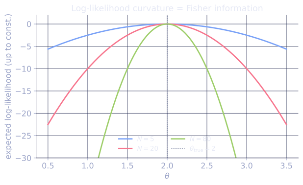
A parameter space is not flat: moving the mean of a sharp Gaussian by 0.1 changes the distribution far more than the same move on a broad one. Fisher information measures this local sensitivity, and treating it as a metric turns the parameter space into a curved geometry where the natural gradient replaces the ordinary one. This is the foundation of efficient estimation and second-order optimization of probabilistic models.

The score and its mean

Recall the score, the gradient of the log-likelihood of a single observation:

Under mild regularity, the score has zero mean at the true parameter:

The densities cancel, the integral is the constant 1, and its gradient is zero.

Fisher information

The Fisher information is the covariance of the score (equivalently, since the score has zero mean, its second moment)[1, 2]:

A second identity rewrites it as the expected negative curvature of the log-likelihood:

Sketch. Differentiate the zero-mean score identity $\int p\,\nabla\log p\,dx = 0$ once more in $\theta$. The product rule produces two terms: $\int (\nabla p)(\nabla \log p)^\top$ and $\int p\,\nabla^2 \log p$. The first equals $\mathbb{E}[s s^\top]$ (using $\nabla p = p\,\nabla\log p$), the second is $\mathbb{E}[\nabla^2 \log p]$, and their sum is zero. Rearranging gives the two forms. High Fisher information means the log-likelihood is sharply peaked, so the parameter is easy to pin down.

This is what makes the opening claim concrete. For a Gaussian with known variance $\sigma^2$ and unknown mean, a single observation carries Fisher information $\mathcal{I} = 1/\sigma^2$. Contrast two models identical except for spread: a sharp $\sigma = 0.2$ gives $\mathcal{I} = 1/0.2^2 = 25$, a broad $\sigma = 2.0$ gives $\mathcal{I} = 1/2.0^2 = 0.25$, a factor of $100$. The same $0.1$ nudge to the mean is $100$ times more distinguishable under the sharp model: the KL between $N(\theta, \sigma^2)$ and $N(\theta + 0.1, \sigma^2)$ is $0.5 \cdot 0.1^2/\sigma^2$, which is $0.125$ for the sharp model and $0.00125$ for the broad one. Sharper densities pack more information about their mean into each sample, so the parameter is pinned down faster.

The Cramer-Rao bound

Fisher information sets the best possible precision of any unbiased estimator $\hat\theta$:

No unbiased estimator beats the inverse Fisher information. The MLE achieves this bound asymptotically, which is the precise sense in which maximum likelihood is efficient.

KL divergence and the Fisher metric

Fisher information is the local curvature of the KL divergence between nearby distributions. A second-order Taylor expansion of $D_{\mathrm{KL}}\big(p_\theta \,\|\, p_{\theta + \delta}\big)$ in the small step $\delta$ gives

with the zeroth and first-order terms vanishing (KL is zero and minimized at $\delta = 0$). So $\mathcal{I}(\theta)$ is the metric tensor that measures distance between distributions in parameter space, the central object of information geometry.

The natural gradient

Ordinary gradient descent steps in the direction of steepest descent measured in Euclidean parameter distance, which is arbitrary: it depends on how the model happens to be parameterized. The natural gradient measures steepest descent in KL distance instead, preconditioning by the inverse Fisher matrix[3]:

Because KL distance is parameterization-invariant, so is the natural-gradient direction. It is the probabilistic cousin of Newton's method (Fisher information in place of the Hessian) and underlies natural-gradient and K-FAC optimizers.

Check it on arrays

import numpy as np

rng = np.random.default_rng(17)

# Gaussian with known variance 1, unknown mean theta.
# log p(x|theta) = -0.5 (x-theta)^2 + const; score = (x - theta); I(theta) = 1.
theta_true = 2.0
N = 2_000_000
x = rng.normal(theta_true, 1.0, N)

score = x - theta_true
print("E[score] ~ 0:", round(score.mean(), 4))
print("Fisher I = Var(score):", round(score.var(), 4), " exact 1.0")

# Curvature form: -E[d^2/dtheta^2 log p] = -E[-1] = 1
print("Fisher (curvature form): 1.0")

# Contrasting pair: sharp vs broad Gaussian, I = 1/sigma^2 per observation
for sigma in [0.2, 2.0]:
    xs = rng.normal(theta_true, sigma, N)
    sc = (xs - theta_true) / sigma**2          # score = (x - theta)/sigma^2
    print(f"sigma={sigma}: Fisher I = Var(score) =", round(sc.var(), 3),
          " exact", 1 / sigma**2)

# Cramer-Rao: MLE (sample mean) variance vs 1/(N*I)
trials = 4000
mle = rng.normal(theta_true, 1.0, size=(trials, 50)).mean(axis=1)
print("Var(MLE) over n=50:", round(mle.var(), 5), " CR bound 1/(n*I) =", round(1/50, 5))

# KL between N(theta,1) and N(theta+d,1) is d^2/2 = 0.5 * d * I * d, with I=1
d = 0.1
kl_exact = d**2 / 2
print("KL(N(0,1)||N(d,1)):", round(kl_exact, 6), " ~ 0.5 d I d:", round(0.5 * d * 1.0 * d, 6))

The score averages to zero, its variance recovers the Fisher information of 1 (and $1/\sigma^2$ for the sharp and broad models, a factor of 100 apart), the MLE variance sits at the Cramer-Rao bound, and the KL between nearby Gaussians equals the Fisher quadratic form.

Exercises

Exercise 1. A single Bernoulli($q$) observation has log-likelihood $\log p(x \mid q) = x \log q + (1 - x)\log(1 - q)$. Use the curvature form $\mathcal{I}(q) = -\mathbb{E}[\partial_q^2 \log p]$ to show that the Fisher information is $\mathcal{I}(q) = \frac{1}{q(1 - q)}$.

Exercise 2. For the Gaussian mean model with known variance $\sigma^2$, a single observation carries Fisher information $\mathcal{I} = 1/\sigma^2$. Show that $n$ i.i.d. observations carry $n/\sigma^2$, and read off the Cramer-Rao bound on the variance of any unbiased estimator of the mean.

Exercise 3 (code). Estimate the Fisher information of a Bernoulli($q$) model by Monte Carlo, using the score-variance form, and confirm it matches the closed form $1/(q(1-q))$ from Exercise 1.

import numpy as np

rng = np.random.default_rng(7)
N = 4_000_000

for q in [0.3, 0.5, 0.7]:
    x = (rng.random(N) < q).astype(float)
    # score of a single Bernoulli obs: x/q - (1-x)/(1-q)
    score = x / q - (1 - x) / (1 - q)
    fisher_mc = score.var()
    fisher_exact = 1.0 / (q * (1 - q))
    print(f"q={q}: Fisher MC = {fisher_mc:.4f}  exact = {fisher_exact:.4f}")
    assert np.isclose(score.mean(), 0.0, atol=2e-3)   # zero-mean score
    assert np.isclose(fisher_mc, fisher_exact, rtol=2e-3)

This closes the A2 probability and information-theory track; the optimization pillar (A3) builds on these gradients and curvatures to actually minimize losses.

References

- [1]Casella, G., & Berger, R. L. (2002). Statistical Inference (2nd ed.). Duxbury. §7.3, Fisher information and the Cramer-Rao lower bound.↩
- [2]Murphy, K. P. (2022). Probabilistic Machine Learning: An Introduction. MIT Press. §4.7, the Fisher information matrix.↩
- [3]Amari, S. (2016). Information Geometry and Its Applications. Springer. The Fisher metric and the natural gradient. doi:10.1007/978-4-431-55978-8↩