Law of large numbers and the central limit theorem

Averaging many independent measurements does two things: it homes in on the true mean, and its leftover error follows a bell curve no matter what the measurements themselves looked like. The law of large numbers is the first statement; the central limit theorem is the second. Together they justify why sampling works and why Gaussian error models are everywhere.

Setup

Let $X_1, X_2, \dots$ be independent and identically distributed (i.i.d.) with mean $\mu = \mathbb{E}[X_i]$ and variance $\sigma^2 = \operatorname{Var}(X_i) < \infty$. The sample mean is

Its own mean and variance follow from linearity and independence:

The mean of the average is the true mean; its variance shrinks like $1/n$.

The weak law of large numbers

Theorem. For any $\varepsilon > 0$, $P(|\bar{X}_n - \mu| \ge \varepsilon) \to 0$ as $n \to \infty$[1].

Proof. Apply Chebyshev to $\bar{X}_n$, which has mean $\mu$ and variance $\sigma^2/n$:

$\qquad\blacksquare$

The sample mean concentrates on $\mu$: for large $n$ it is within any fixed tolerance with probability approaching 1. This is the formal reason Monte Carlo estimates converge to the quantity they estimate.

The central limit theorem

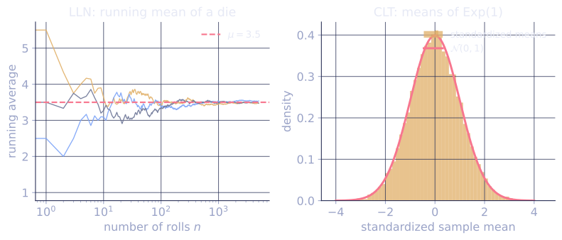
The LLN says the error $\bar{X}_n - \mu$ vanishes; the CLT describes its shape after rescaling so it does not. Since the error has standard deviation $\sigma/\sqrt n$, multiply by $\sqrt n / \sigma$ to keep it order 1.

Theorem. As $n \to \infty$[2],

where $\xrightarrow{d}$ means the CDF converges to that of the standard normal at every point.

The remarkable part is universality: the limit is $\mathcal{N}(0,1)$ regardless of the distribution of the $X_i$, requiring only finite variance. The MGF gives the intuition: the standardized sum's MGF is the $n$-th power of a single term's MGF, and $\big(1 + \frac{t^2}{2n} + o(1/n)\big)^n \to e^{t^2/2}$, the MGF of the standard normal. A matching MGF means a matching distribution.

Equivalently, for large $n$ the sample mean is approximately $\bar{X}_n \approx \mathcal{N}(\mu, \sigma^2/n)$. This is the basis of confidence intervals: $\bar{X}_n \pm 1.96\,\sigma/\sqrt n$ contains $\mu$ about 95% of the time.

Check it on arrays

import numpy as np

rng = np.random.default_rng(10)

# LLN: running mean of a fair die converges to 3.5
draws = rng.integers(1, 7, size=100_000).astype(float)
running = np.cumsum(draws) / np.arange(1, len(draws) + 1)
for n in [10, 100, 1000, 100_000]:
    print(f"n={n:>6}: running mean {running[n-1]:.4f}  (target 3.5)")

# CLT: standardized sample means of a *skewed* exponential become Gaussian
n, trials = 1000, 200_000
mu, sigma = 1.0, 1.0                       # Exponential(rate=1): mean=var=1
samples = rng.exponential(1.0, size=(trials, n))
means = samples.mean(axis=1)
standardized = (means - mu) / (sigma / np.sqrt(n))
print("standardized sample-mean: mean", round(standardized.mean(), 3),
      "std", round(standardized.std(), 3))
# Fraction within 1.96 should be ~0.95
print("frac within +/-1.96:", round(np.mean(np.abs(standardized) < 1.96), 4))

The running die average settles onto 3.5, and the standardized means of a skewed exponential become a unit normal with ~95% of mass inside $\pm1.96$.

Exercises

Exercise 1. A fair die has mean $\mu = 3.5$ and variance $\sigma^2 = 35/12 \approx 2.9167$. For $n = 100$ rolls, use Chebyshev's inequality (as in the LLN proof) to bound the probability that the sample mean deviates from $3.5$ by at least $0.5$.

Exercise 2. The CLT says $\bar X_n \approx \mathcal{N}(\mu, \sigma^2/n)$. Using the standard normal fact $P(|Z| \le 1.96) \approx 0.95$, derive the width of a 95% confidence interval for $\mu$ and show how it shrinks with $n$.

Exercise 3 (code). Take the most skewed start possible, a Bernoulli($0.1$) variable. Verify the LLN (running mean converges to $0.1$) and the CLT (standardized sample means over $n = 500$ are approximately standard normal, with about 95% of mass within $\pm 1.96$).

import numpy as np

rng = np.random.default_rng(11)

p = 0.1
mu, sigma = p, np.sqrt(p * (1 - p))    # Bernoulli mean and std

# LLN: running mean of Bernoulli(0.1) converges to 0.1
draws = (rng.random(200_000) < p).astype(float)
running = np.cumsum(draws) / np.arange(1, len(draws) + 1)
assert abs(running[-1] - p) < 0.01

# CLT: standardized means over n=500 are ~ N(0,1)
n, trials = 500, 200_000
samples = (rng.random((trials, n)) < p).astype(float)
means = samples.mean(axis=1)
z = (means - mu) / (sigma / np.sqrt(n))
frac = np.mean(np.abs(z) < 1.96)
assert abs(z.mean()) < 0.02 and abs(z.std() - 1.0) < 0.02
assert abs(frac - 0.95) < 0.01
print("running mean:", round(running[-1], 4), " frac within 1.96:", round(frac, 4))

With sampling behavior pinned down, the next lesson uses it in reverse: estimating a distribution's parameters from data by maximum likelihood.

References

- [1]Wasserman, L. (2004). All of Statistics. Springer. Ch. 5, the law of large numbers and convergence of random variables. doi:10.1007/978-0-387-21736-9↩
- [2]Durrett, R. (2019). Probability: Theory and Examples (5th ed.). Cambridge University Press. Ch. 3, the central limit theorem.↩