Bernoulli, Binomial, Poisson, Gaussian

A handful of distributions show up again and again because each models a simple, recurring mechanism: a single yes/no trial, a count of successes, a count of rare events, and the limiting bell curve that sums of anything tend toward[1]. Knowing their stories and moments cold pays off everywhere downstream.

Bernoulli: one trial

A Bernoulli random variable $X \in \{0, 1\}$ models a single trial with success probability $q$:

Mean: $\mathbb{E}[X] = 1 \cdot q + 0 \cdot (1-q) = q$. Variance: $\mathbb{E}[X^2] = q$ (since $X^2 = X$ for a 0/1 variable), so $\operatorname{Var}(X) = q - q^2 = q(1-q)$, maximized at $q = 1/2$.

Binomial: counting successes

The Binomial $X \sim \text{Bin}(n, q)$ counts successes in $n$ independent Bernoulli($q$) trials. The PMF multiplies the probability of any specific sequence with $k$ successes, $q^k(1-q)^{n-k}$, by the number of such sequences:

Writing $X = \sum_{i=1}^n X_i$ as a sum of independent Bernoullis, linearity and (for independent terms) additivity of variance give

with no need to sum the PMF directly. The sum-of-indicators decomposition is the fast route to both moments.

Poisson: rare events

The Poisson $X \sim \text{Pois}(\lambda)$ counts events in a fixed interval when they occur independently at an average rate $\lambda$. It arises as the limit of $\text{Bin}(n, \lambda/n)$ as $n \to \infty$ (many trials, each rarely succeeding):

A defining feature is equal mean and variance:

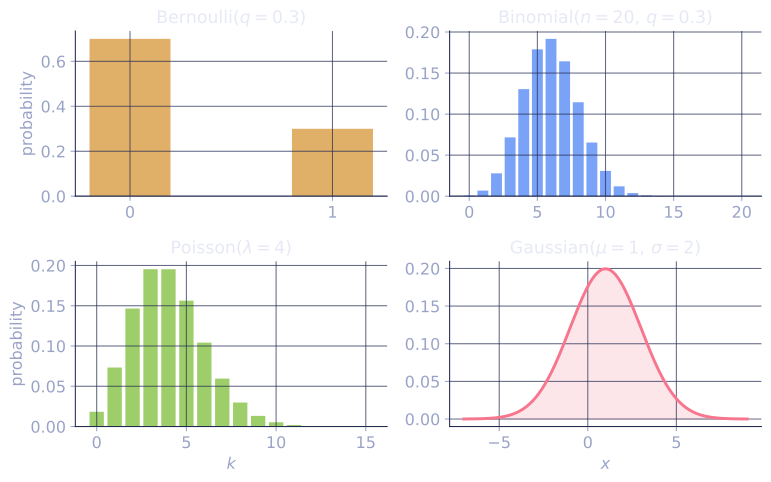
This equality is a quick diagnostic: count data with variance much larger than its mean is "overdispersed" and not Poisson. The mean-variance relationship separates these count distributions sharply, using the parameters from the code below:

• Binomial(20, 0.3) has mean $nq = 6$ but variance $nq(1-q) = 4.2$. The variance sits below the mean, because a bounded count ($0 \le k \le 20$) cannot spread freely.
• Poisson(4) has mean and variance both equal to $4$. Removing the upper bound (Poisson counts run to infinity) lets the variance rise to match the mean.

So variance below the mean points to a bounded Binomial-like count, variance equal to the mean to a Poisson, and variance above the mean to overdispersion that neither models.

Gaussian: the bell curve

The Gaussian (normal) $X \sim \mathcal{N}(\mu, \sigma^2)$ is the continuous distribution with PDF[2]

Its parameters are its moments directly: $\mathbb{E}[X] = \mu$ and $\operatorname{Var}(X) = \sigma^2$. The standard normal $\mathcal{N}(0, 1)$ has $\mu = 0, \sigma = 1$, and any Gaussian standardizes via $Z = (X - \mu)/\sigma$.

The Gaussian dominates because of the central limit theorem (a later lesson): sums and averages of many independent contributions converge to it regardless of the pieces' own distributions. Sums of independent Gaussians are again Gaussian, with means and variances adding.

Check it on arrays

import numpy as np
from math import comb, factorial

rng = np.random.default_rng(6)
N = 1_000_000

# Bernoulli(0.3)
q = 0.3
B = (rng.random(N) < q).astype(float)
print(f"Bernoulli mean {B.mean():.3f} (q={q}), var {B.var():.3f} (q(1-q)={q*(1-q):.3f})")

# Binomial(n=20, q=0.3)
n = 20
X = rng.binomial(n, q, size=N)
print(f"Binomial mean {X.mean():.3f} (nq={n*q}), var {X.var():.3f} (nq(1-q)={n*q*(1-q):.3f})")
# Check one PMF value
k = 6
print(f"P(X={k}) sim {np.mean(X == k):.4f}, exact {comb(n,k)*q**k*(1-q)**(n-k):.4f}")

# Poisson(lambda=4): mean == variance
lam = 4.0
Pn = rng.poisson(lam, size=N)
print(f"Poisson mean {Pn.mean():.3f}, var {Pn.var():.3f} (both {lam})")
print(f"P(X=3) sim {np.mean(Pn == 3):.4f}, exact {lam**3*np.exp(-lam)/factorial(3):.4f}")

# Gaussian(mu=1, sigma=2): standardize and check ~N(0,1)
G = rng.normal(1.0, 2.0, size=N)
Z = (G - 1.0) / 2.0
print(f"standardized mean {Z.mean():.3f} (~0), std {Z.std():.3f} (~1)")

Every mean and variance lands on its formula, the binomial and Poisson PMF spot checks match, and standardizing the Gaussian produces a unit normal.

Exercises

Exercise 1. A fair die is rolled 12 times. Model the number of sixes as a Binomial and compute its mean and variance from the formulas, then give $P(X = 2)$ to four decimals.

Exercise 2. Take the Binomial $\text{Bin}(n, \lambda/n)$ and show that, as $n \to \infty$ with $\lambda$ fixed, its PMF at a fixed $k$ converges to the Poisson PMF $\frac{\lambda^k e^{-\lambda}}{k!}$.

Exercise 3 (code). Demonstrate the convergence of Exercise 2 numerically: compare the $\text{Bin}(n, 4/n)$ PMF against $\text{Pois}(4)$ at $k = 0, \dots, 9$ for growing $n$, and confirm the gap shrinks.

import numpy as np
from math import comb, factorial

lam = 4.0
ks = np.arange(10)

def binom_pmf(n, q, k):
    return comb(n, k) * q**k * (1 - q)**(n - k)

def pois_pmf(lam, k):
    return lam**k * np.exp(-lam) / factorial(k)

pois = np.array([pois_pmf(lam, k) for k in ks])

prev = None
for n in [10, 50, 200, 1000]:
    binom = np.array([binom_pmf(n, lam / n, k) for k in ks])
    err = np.max(np.abs(binom - pois))
    print(f"n={n:5d}  max |Bin - Pois| = {err:.5f}")
    if prev is not None:
        assert err < prev          # error decreases as n grows
    prev = err

The next lesson shows that three of these four share a single algebraic skeleton: the exponential family.