Shannon entropy

How much uncertainty is in a distribution? A fair coin is more uncertain than a biased one; a uniform die more than a loaded one. Shannon entropy turns this intuition into a number, measured in bits, and it is the floor on how many bits per symbol any lossless code can achieve[1, 2]. It is also the backbone of the cross-entropy loss.

Surprise

The surprise (or information content) of an outcome with probability $p$ is

Three requirements force this form. Surprise should decrease in $p$ (certain events are unsurprising, $I(1) = 0$), be nonnegative, and be additive for independent events: seeing two independent outcomes of probability $p_1, p_2$ should surprise you by $I(p_1) + I(p_2)$. Since the joint probability is $p_1 p_2$, the function must satisfy $I(p_1 p_2) = I(p_1) + I(p_2)$, and the logarithm is the function that turns products into sums. With $\log_2$, surprise is in bits.

A good mental hook: surprise measures newsworthiness, how much you learn when one specific outcome actually happens. Some real-world magnitudes:

• The sun rose this morning. $p \approx 1$, so $I \approx 0$ bits. You learned nothing; nobody reports it.
• A fair coin landed heads. $p = 1/2$, so $I = 1$ bit, the unit itself.
• Two dice came up snake eyes. $p = 1/36$, so $I = \log_2 36 \approx 5.2$ bits. Noteworthy at the table, not in the paper.
• You won a national lottery. $p \approx 3 \times 10^{-9}$ (about one in 300 million), so $I \approx 28$ bits. Front-page news, precisely because it was so improbable.

The additivity requirement is easy to sanity-check on the coin: two heads in a row has probability $\tfrac12 \cdot \tfrac12 = \tfrac14$, and your surprise is $1 + 1 = 2$ bits; indeed $-\log_2 \tfrac14 = 2$. And a "bit" itself has an operational reading: an event of probability $1/8$ carries $\log_2 8 = 3$ bits because learning it happened is like learning which of $8$ equally likely doors opened, which takes exactly three yes/no questions.

Entropy

The entropy of a discrete distribution $p$ is the expected surprise[3]:

with the convention $0 \log 0 = 0$ (vanishingly rare outcomes contribute nothing). With $\log_2$ it is in bits; with natural log, in nats. Entropy is a property of the distribution, not of any particular outcome: it asks not "how surprised am I by this event?" but "how surprised am I on average, draw after draw?"

Compare the weather in two cities. In a desert city, $P(\text{sun}) = 0.99$ and $P(\text{rain}) = 0.01$. Almost every morning you look outside and learn essentially nothing ($I \approx 0.014$ bits); once in a hundred days you are quite surprised ($I = \log_2 100 \approx 6.6$ bits), but that almost never happens. The average is

The weather there is boring: low entropy. In a coin-flip city with $P(\text{sun}) = P(\text{rain}) = 0.5$, every single morning is a genuine coin toss worth one full bit: $H = 1$ bit, the most unpredictable a two-outcome source can be.

This averaging resolves a confusion worth naming explicitly: a rare event has huge surprise but contributes almost nothing to entropy, because entropy weights each surprise by how often it occurs, and $p \log\frac{1}{p} \to 0$ as $p \to 0$ (that is exactly the $0 \log 0 = 0$ convention at work). The lottery is the extreme case: winning is a 28-bit shock, yet the lottery as a distribution has nearly zero entropy (about $10^{-7}$ bits), because the outcome is almost always the utterly unsurprising "you lost." High surprise describes one outcome; high entropy describes an unpredictable source. They can point in opposite directions.

The binary entropy function

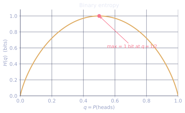
For a Bernoulli($q$) variable,

It is 0 at $q = 0$ and $q = 1$ (no uncertainty) and peaks at $q = 1/2$ with $H(1/2) = 1$ bit. A fair coin carries exactly one bit; any bias reduces it.

Bounds

Entropy is nonnegative: each term $-p(x)\log p(x) \ge 0$ because $0 \le p(x) \le 1$ makes $\log p(x) \le 0$.

Maximum at the uniform distribution. Among all distributions on $K$ outcomes, entropy is largest for the uniform $p(x) = 1/K$, where $H = \log K$. This follows from Jensen's inequality applied to the concave $\log$:

Equality holds when $1/p(X)$ is constant, i.e. $p$ is uniform. Uncertainty is maximized when no outcome is favored.

Differential entropy

For a continuous density $f$, the analogue is the differential entropy $h(X) = -\int f(x)\log f(x)\,dx$. It can be negative and is not invariant under change of variables (a coordinate stretch shifts it by the log-Jacobian), so it behaves differently from discrete entropy. Among densities with a fixed variance $\sigma^2$, the Gaussian maximizes differential entropy at $\frac{1}{2}\log(2\pi e\sigma^2)$, a reason the Gaussian is the "least assuming" choice at fixed spread.

Check it on arrays

import numpy as np

# Binary entropy peaks at q = 0.5
def H_bits(p):
    p = np.asarray(p, float)
    nz = p[p > 0]                       # skip zero-probability outcomes
    return -np.sum(nz * np.log2(nz))

for q in [0.0, 0.1, 0.5, 0.9, 0.99, 1.0]:    # 0.99 = the desert city
    dist = np.array([q, 1 - q])
    print(f"H(Bernoulli({q})) = {H_bits(dist):.4f} bits")

# Uniform over K outcomes has entropy log2(K); it is the maximum
K = 8
uniform = np.full(K, 1 / K)
skewed = np.array([0.5] + [0.5 / (K - 1)] * (K - 1))
print(f"H(uniform_{K}) = {H_bits(uniform):.4f} (log2 {K} = {np.log2(K):.4f})")
print(f"H(skewed)    = {H_bits(skewed):.4f}  (< uniform)")

# Entropy as expected surprise, estimated from samples
rng = np.random.default_rng(13)
probs = np.array([0.5, 0.25, 0.15, 0.10])
samples = rng.choice(len(probs), size=500_000, p=probs)
surprise = -np.log2(probs[samples])
print("E[surprise] sampled:", round(surprise.mean(), 4),
      " true H:", round(H_bits(probs), 4))

The binary entropy peaks at one bit for a fair coin, the uniform distribution attains the maximum $\log_2 K$, and average sampled surprise matches the entropy.

Exercises

Exercise 1. Compute, by hand, the entropy in bits of $p = \left(\tfrac12, \tfrac14, \tfrac18, \tfrac18\right)$.

Exercise 2. Let $X$ and $Y$ be independent discrete variables. Prove that entropy is additive: $H(X, Y) = H(X) + H(Y)$, where $H(X, Y)$ is the entropy of the pair $(X, Y)$ under the joint distribution.

Exercise 3 (code). Draw 10,000 random distributions on $K = 4$ outcomes (normalize positive random vectors). Verify numerically that none exceeds $\log_2 4 = 2$ bits, and that the entropy of Exercise 1's distribution is exactly $1.75$ bits.

import numpy as np

def H_bits(p):
    p = np.asarray(p, float)
    nz = p[p > 0]
    return -np.sum(nz * np.log2(nz))

rng = np.random.default_rng(0)
raw = rng.random((10_000, 4))
dists = raw / raw.sum(axis=1, keepdims=True)   # rows sum to 1
ents = np.array([H_bits(d) for d in dists])

assert ents.max() <= 2.0                        # Jensen bound: H <= log2 K
assert np.isclose(H_bits([0.5, 0.25, 0.125, 0.125]), 1.75)
print("max sampled H:", round(ents.max(), 4), "of bound", 2.0)

The next lesson compares two distributions instead of summarizing one: the KL divergence.

References

- [1]Shannon, C. E. (1948). "A mathematical theory of communication". Bell System Technical Journal, 27, 379-423. The paper that introduced entropy and the noiseless source coding bound. doi:10.1002/j.1538-7305.1948.tb01338.x↩
- [2]Cover, T. M., & Thomas, J. A. (2006). Elements of Information Theory (2nd ed.). Wiley. Ch. 2, entropy and the source coding theorem. doi:10.1002/047174882X↩
- [3]MacKay, D. J. C. (2003). Information Theory, Inference, and Learning Algorithms. Cambridge University Press. Ch. 2-4, surprise, entropy, and Shannon information.↩