MAP estimation and conjugate priors

Maximum likelihood trusts the data alone. When data are scarce or you hold prior belief about a parameter, Bayesian inference combines both: it treats the parameter as random, places a prior on it, and updates to a posterior[1]. Conjugate priors keep that update in closed form, and MAP estimation reads off its peak.

The posterior over parameters

Treat the parameter $\theta$ as a random variable with prior density $p(\theta)$. Bayes' rule gives the posterior after observing data $\mathcal{D}$:

The evidence $p(\mathcal{D}) = \int p(\mathcal{D} \mid \theta)p(\theta)\,d\theta$ is a constant in $\theta$, so for finding the shape (and the peak) of the posterior it can be ignored: posterior $\propto$ likelihood $\times$ prior.

MAP estimation

The maximum a posteriori (MAP) estimate is the posterior mode:

It is maximum likelihood plus an additive prior term. With a Gaussian prior on weights, $\log p(\theta) = -\frac{1}{2\tau^2}\lVert\theta\rVert^2 + \text{const}$, and MAP becomes likelihood maximization with an L2 (ridge) penalty. A Laplace prior gives an L1 penalty. Regularization is a prior in disguise.

As data accumulate, the likelihood term grows with $n$ while the prior term stays fixed, so the MAP estimate converges to the MLE: the prior washes out.

Conjugate priors

A prior is conjugate to a likelihood if the posterior belongs to the same family as the prior[2]. Then updating only changes the family's parameters, with no integration required.

Beta-Bernoulli. For $n$ Bernoulli($q$) trials with $k$ successes, the likelihood is $q^k(1-q)^{n-k}$. The conjugate prior is the Beta distribution $p(q) \propto q^{\alpha-1}(1-q)^{\beta-1}$. Multiplying,

which is $\text{Beta}(\alpha + k,\ \beta + n - k)$. The update just adds successes to $\alpha$ and failures to $\beta$. The prior parameters act as pseudo-counts: prior belief stated as "as if I had already seen $\alpha$ successes and $\beta$ failures".

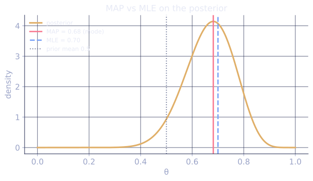
The posterior mean and mode are

The MAP mode reduces to the MLE $k/n$ when $\alpha = \beta = 1$ (a flat prior).

Check it on arrays

import numpy as np

rng = np.random.default_rng(12)

# True coin bias, small sample so the prior matters
true_q = 0.7
n = 20
data = (rng.random(n) < true_q).astype(int)
k = data.sum()
print(f"observed {k} heads in {n} flips; MLE = {k/n:.3f}")

# Beta(2,2) prior (mild belief near 0.5), conjugate update
alpha0, beta0 = 2.0, 2.0
alpha_post, beta_post = alpha0 + k, beta0 + (n - k)
post_mean = alpha_post / (alpha_post + beta_post)
post_mode = (alpha_post - 1) / (alpha_post + beta_post - 2)
print(f"posterior Beta({alpha_post}, {beta_post})")
print(f"posterior mean {post_mean:.3f}, MAP mode {post_mode:.3f}")

# Verify conjugacy numerically: posterior ∝ likelihood * prior on a grid
q = np.linspace(1e-3, 1 - 1e-3, 5000)
dq = q[1] - q[0]
prior = q**(alpha0 - 1) * (1 - q)**(beta0 - 1)
like = q**k * (1 - q)**(n - k)
post = prior * like
post /= post.sum() * dq                          # normalize (Riemann sum)
beta_pdf = q**(alpha_post - 1) * (1 - q)**(beta_post - 1)
beta_pdf /= beta_pdf.sum() * dq
print("max |grid posterior - Beta pdf|:", round(np.max(np.abs(post - beta_pdf)), 6))
print("grid MAP:", round(q[np.argmax(post)], 3))

The conjugate update gives a Beta posterior whose density matches the likelihood-times-prior computed on a grid, and the MAP mode pulls the estimate toward the prior on this small sample.

Exercises

Exercise 1. Start from a $\text{Beta}(2, 2)$ prior on a coin's bias $q$. You observe $8$ heads in $10$ flips. Give the posterior distribution and compute its mean and MAP mode.

Exercise 2. Show that with a flat $\text{Beta}(1, 1)$ prior, the MAP mode equals the MLE $k/n$, and explain why this is the prior that adds no information.

Exercise 3 (code). Confirm the conjugate update numerically. Compute the normalized likelihood-times-prior on a grid for the Exercise 1 setting, and check that its mode matches the closed-form MAP $0.75$ and its mean matches $5/7$.

import numpy as np

alpha0, beta0 = 2.0, 2.0
k, n = 8, 10

q = np.linspace(1e-4, 1 - 1e-4, 200_000)
dq = q[1] - q[0]
prior = q**(alpha0 - 1) * (1 - q)**(beta0 - 1)
like = q**k * (1 - q)**(n - k)
post = prior * like
post /= post.sum() * dq                    # normalize (Riemann sum)

grid_mode = q[np.argmax(post)]
grid_mean = (q * post).sum() * dq

assert np.isclose(grid_mode, 0.75, atol=1e-3)
assert np.isclose(grid_mean, 5 / 7, atol=1e-3)
print("grid MAP:", round(grid_mode, 4), " grid mean:", round(grid_mean, 4))

The next lesson shifts from estimating distributions to quantifying their information content, starting with entropy.