Transformations of random variables

You often know the distribution of $X$ but need the distribution of $Y = g(X)$: sampling a uniform and turning it into a Gaussian, or pushing a latent variable through a neural network in a normalizing flow. The change-of-variables formula tells you exactly how a density transforms, and the determinant from linear algebra reappears as the local volume-stretching factor.

The CDF route (always works)

The safe, general method is to compute the CDF of $Y$ and differentiate. For an increasing $g$,

Differentiating with the chain rule gives the density. This route handles non-monotone $g$ too, by splitting into monotone pieces.

The change-of-variables formula (1D)

For a differentiable, strictly monotone $g$ with inverse $x = g^{-1}(y)$, differentiating $F_Y(y) = F_X(g^{-1}(y))$[1]:

The absolute value covers decreasing $g$ (where $F_Y(y) = 1 - F_X(g^{-1}(y))$, and the derivative is negative). The factor $|dg^{-1}/dy|$ corrects for how $g$ stretches or compresses the axis: where $g$ spreads probability over a wider range, the density thins out.

A useful restatement uses $dy/dx = g'(x)$:

Probability mass is conserved, $f_Y(y)\,|dy| = f_X(x)\,|dx|$; only its density per unit length changes.

The multivariate formula

For an invertible differentiable map $\mathbf{y} = g(\mathbf{x})$ on $\mathbb{R}^n$, the single derivative becomes the Jacobian determinant[2]:

where $J_{g^{-1}}$ is the Jacobian matrix of the inverse map. The determinant is the local volume-scaling factor of the transformation (its meaning from linear algebra), now applied pointwise to a nonlinear map. This is the identity normalizing flows exploit: stack invertible maps with cheap log-determinants to build a flexible density whose normalization stays tractable.

Worked example: inverse-CDF sampling

If $U \sim \text{Uniform}(0,1)$ and $F$ is a target CDF, then $X = F^{-1}(U)$ has CDF $F$. Check it:

using that $F$ is increasing and $U$ is uniform on $[0,1]$ (so $P(U \le u) = u$). This is how a single uniform random source generates samples from any distribution with an invertible CDF, for example the exponential via $X = -\frac{1}{\lambda}\log(1-U)$.

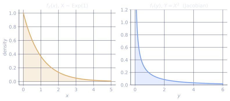
Check it on arrays

import numpy as np

rng = np.random.default_rng(8)
N = 1_000_000

# Inverse-CDF sampling for Exponential(rate=lambda): X = -ln(1-U)/lambda
lam = 1.5
U = rng.random(N)
X = -np.log(1 - U) / lam
print("inverse-CDF exp mean:", round(X.mean(), 4), "  exact 1/lambda =", round(1/lam, 4))
print("numpy exp mean:      ", round(rng.exponential(1/lam, N).mean(), 4))

# Change of variables: Y = X^2 for X ~ N(0,1); density check via histogram
Xn = rng.normal(size=N)
Y = Xn**2                                   # chi-square with 1 dof
hist, edges = np.histogram(Y, bins=200, range=(0.01, 5), density=True)
centers = 0.5 * (edges[:-1] + edges[1:])
# f_Y(y) = f_X(sqrt y)/|g'(x)| summed over the two roots +/-sqrt(y):
#        = 2 * phi(sqrt y) * (1/(2 sqrt y)) = phi(sqrt y)/sqrt y
phi = lambda x: np.exp(-x**2/2)/np.sqrt(2*np.pi)
f_theory = phi(np.sqrt(centers)) / np.sqrt(centers)
print("max |hist - theory|:", round(np.max(np.abs(hist - f_theory)), 4))

Inverse-CDF sampling reproduces the exponential mean, and the analytic density of $X^2$ (with the Jacobian factor and both roots accounted for) matches its histogram.

Exercises

Exercise 1. Let $X \sim \text{Uniform}(0, 1)$ and $Y = -\log X$. Use the 1D change-of-variables formula to find the density $f_Y(y)$ and name the resulting distribution.

Exercise 2. Let $X$ have density $f_X$ and let $Y = aX + b$ with $a \ne 0$, an affine transform. Derive $f_Y(y)$ and confirm it specializes correctly: a Gaussian $X \sim \mathcal{N}(\mu, \sigma^2)$ maps to $\mathcal{N}(a\mu + b, a^2\sigma^2)$.

Exercise 3 (code). Verify Exercise 1 numerically: transform a million uniform samples by $Y = -\log X$ and confirm the empirical histogram matches the Exponential(1) density $e^{-y}$.

import numpy as np

rng = np.random.default_rng(0)
N = 1_000_000

X = rng.random(N)
Y = -np.log(X)

hist, edges = np.histogram(Y, bins=200, range=(0.0, 6.0), density=True)
centers = 0.5 * (edges[:-1] + edges[1:])
f_theory = np.exp(-centers)        # Exponential(1) density

max_err = np.max(np.abs(hist - f_theory))
print("mean of Y:", round(Y.mean(), 4), " exact 1.0")
print("max |hist - theory|:", round(max_err, 4))
assert np.isclose(Y.mean(), 1.0, atol=1e-2)
assert max_err < 0.02

The next lesson steps back from exact distributions to bounds that hold for all of them: the basic probability inequalities.

References

- [1]Casella, G., & Berger, R. L. (2002). Statistical Inference (2nd ed.). Duxbury. §2.1, distributions of functions of a random variable.↩
- [2]Wasserman, L. (2004). All of Statistics. Springer. §2.7-2.8, transformations of random variables and the multivariate Jacobian. doi:10.1007/978-0-387-21736-9↩