Joint, marginal, and conditional distributions

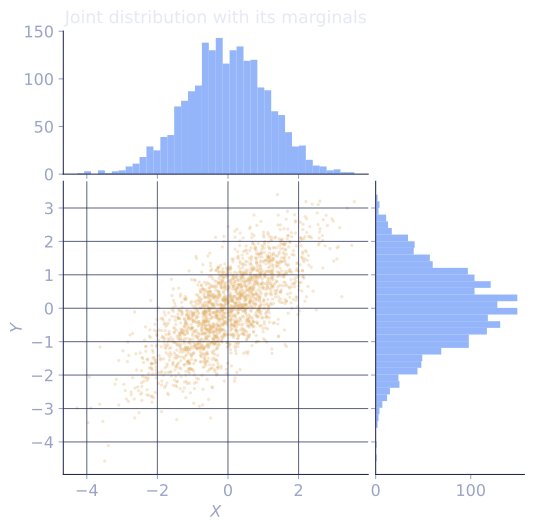
Most interesting questions involve more than one quantity at once: a pixel and its neighbor, a feature and a label, today's price and tomorrow's. The joint distribution describes how two random variables vary together, and from it come the two operations at the heart of probabilistic modeling: marginalizing and conditioning[1].

Joint distribution

For two discrete random variables $X, Y$, the joint PMF is

the probability that both take their stated values. It is nonnegative and sums to 1 over all pairs. The continuous analogue is a joint PDF $f_{X,Y}(x, y)$ with $\iint f_{X,Y} = 1$, where probabilities come from integrating over a region.

Marginalization

To recover the distribution of one variable alone, sum (or integrate) the joint over the other. The marginal PMF of $X$ is

Why. The event $\{X = x\}$ is the disjoint union over all $y$ of the events $\{X = x, Y = y\}$. Countable additivity turns that union into the sum above. Marginalizing is summing out the variables you do not care about.

Conditional distribution

The conditional PMF of $Y$ given $X = x$ rescales the slice of the joint at $X = x$ so it sums to 1:

This is the definition $P(A \mid B) = P(A \cap B)/P(B)$ written for random variables. Conditioning answers "given that I have observed $X = x$, how is $Y$ distributed?" The denominator $p_X(x)$ is exactly the marginal, which is why it is the normalizing constant of the slice.

Rearranged, the definition gives the chain rule for distributions:

A joint factors into a marginal times a conditional, the basic move behind every generative model.

Independence

$X$ and $Y$ are independent if the joint factors into the product of marginals for all values[2]:

Equivalently, $p_{Y \mid X}(y \mid x) = p_Y(y)$: knowing $X$ tells you nothing about $Y$. Independence is a strong assumption, and the factorization is what makes likelihoods of independent samples multiply.

Covariance

The covariance measures the linear co-movement of two variables:

The second form follows by expanding and using linearity, exactly as in the single-variable variance formula. Positive covariance means they tend to move together; negative means opposite; and independence implies zero covariance (since then $\mathbb{E}[XY] = \mathbb{E}[X]\mathbb{E}[Y]$). The converse fails: zero covariance does not imply independence, because covariance only sees linear structure.

That last point names a confusion worth pinning to a concrete case, since "zero covariance" and "independent" are routinely treated as the same thing. Take $X$ uniform on $\{-1, 0, 1\}$ and set $Y = X^2$. Here $Y$ is a deterministic function of $X$ (the strongest possible dependence: observe $X$ and you know $Y$ exactly), yet $\mathbb{E}[X] = 0$, $\mathbb{E}[XY] = \mathbb{E}[X^3] = 0$, so $\operatorname{Cov}(X, Y) = 0 - 0 \cdot \tfrac{2}{3} = 0$. The covariance is blind to this dependence because the dependence is curved, not linear: $X$ and $-X$ contribute opposite-signed cross terms that cancel. Zero covariance rules out linear co-movement, nothing more.

The variance of a sum picks up a covariance term:

For independent variables the cross term vanishes and variances simply add.

Check it on arrays

import numpy as np

rng = np.random.default_rng(4)
N = 500_000

# Correlated pair via a shared component
Z = rng.normal(size=N)
X = Z + rng.normal(size=N) * 0.5
Y = Z - rng.normal(size=N) * 0.5

cov = np.mean((X - X.mean()) * (Y - Y.mean()))
print("Cov(X, Y):", round(cov, 4), "  (positive: shared Z)")

# Var(X + Y) = Var(X) + Var(Y) + 2 Cov(X, Y)
lhs = (X + Y).var()
rhs = X.var() + Y.var() + 2 * cov
print("Var(X+Y):", round(lhs, 4), "  decomposition:", round(rhs, 4))

# Independent pair: covariance ~ 0
U = rng.normal(size=N)
V = rng.normal(size=N)
print("Cov(indep):", round(np.mean((U - U.mean()) * (V - V.mean())), 4))

# Dependent yet zero-covariance: X uniform on {-1,0,1}, Y = X^2 (Y is a function of X)
Xd = rng.integers(-1, 2, size=N)        # -1, 0, or 1
Yd = Xd**2
print("Cov(X, X^2):", round(np.mean((Xd - Xd.mean()) * (Yd - Yd.mean())), 4), " (~0, yet dependent)")

# Marginal by summing a joint table (discrete)
joint = np.array([[0.1, 0.2], [0.3, 0.4]])   # P(X=i, Y=j)
print("P(X) marginal:", joint.sum(axis=1))   # sum over Y
print("P(Y|X=0):", joint[0] / joint[0].sum())

The covariance is positive for the shared-component pair, the variance-of-sum decomposition holds, the independent pair has near-zero covariance, the function-dependent pair $(X, X^2)$ also has near-zero covariance despite being fully dependent, and summing a joint table recovers the marginal.

Exercises

Exercise 1. The joint PMF of $(X, Y)$ is given by the table below, with $X$ the row index and $Y$ the column index.

Compute the marginal $p_X$, the conditional $p_{Y \mid X}(y \mid 1)$, and decide whether $X$ and $Y$ are independent.

Exercise 2. Let $X$ and $Y$ be independent with $\operatorname{Var}(X) = 4$ and $\operatorname{Var}(Y) = 9$. Compute $\operatorname{Var}(2X - Y)$.

Exercise 3 (code). Build a $3 \times 3$ joint table by normalizing a random nonnegative matrix. Then verify on samples drawn from it that the empirical conditional $p(Y \mid X = 0)$ matches the table's conditional, and that $\mathbb{E}[XY] - \mathbb{E}[X]\mathbb{E}[Y]$ recovers the covariance computed directly from the table.

import numpy as np

rng = np.random.default_rng(3)
vals = np.array([0, 1, 2], dtype=float)

raw = rng.random((3, 3))
joint = raw / raw.sum()                       # P(X=i, Y=j), sums to 1

# Table conditional P(Y | X=0)
cond_table = joint[0] / joint[0].sum()

# Sample (X, Y) pairs from the flattened joint
flat = joint.ravel()
idx = rng.choice(9, size=2_000_000, p=flat)
Xs, Ys = idx // 3, idx % 3
cond_emp = np.array([np.mean(Ys[Xs == 0] == j) for j in range(3)])
assert np.allclose(cond_table, cond_emp, atol=2e-3)

# Covariance from the table vs E[XY] - E[X]E[Y]
EX = (joint.sum(axis=1) * vals).sum()
EY = (joint.sum(axis=0) * vals).sum()
EXY = sum(joint[i, j] * vals[i] * vals[j] for i in range(3) for j in range(3))
cov_table = EXY - EX * EY
cov_emp = np.mean(vals[Xs] * vals[Ys]) - vals[Xs].mean() * vals[Ys].mean()
assert np.isclose(cov_table, cov_emp, atol=5e-3)
print("cond match:", np.round(cond_table, 4))
print("cov table:", round(cov_table, 4), " sampled:", round(cov_emp, 4))

The next lesson turns the conditioning formula around into Bayes' rule.

References

- [1]Wasserman, L. (2004). All of Statistics. Springer. Ch. 2-3, joint, marginal, and conditional distributions. doi:10.1007/978-0-387-21736-9↩
- [2]Bishop, C. M. (2006). Pattern Recognition and Machine Learning. Springer. §1.2, the sum and product rules and independence.↩