Variance, moments, and moment generating functions

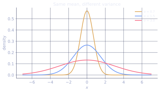
The mean says where a distribution sits; it says nothing about how spread out it is. Two distributions with the same mean can be a tight spike or a broad smear. Variance measures that spread, and the moment generating function packages the mean, variance, and every higher moment into a single function.

Variance and standard deviation

The variance of $X$ is the expected squared deviation from the mean $\mu = \mathbb{E}[X]$[1]:

Squaring makes deviations positive and penalizes large ones more. The standard deviation $\sigma = \sqrt{\operatorname{Var}(X)}$ returns to the original units.

A feel for the scale, on familiar spreads:

• Adult heights scatter with $\sigma \approx 7$ cm, so $\operatorname{Var} = 49\ \text{cm}^2$.
• IQ scores are built to $\sigma = 15$ points, so $\operatorname{Var} = 225\ \text{points}^2$.
• A tight instrument reading with $\sigma = 0.1$ has $\operatorname{Var} = 0.01$.

The squared units expose a confusion worth naming: variance and standard deviation are not interchangeable, because they live in different units. Variance is in squared units (cm$^2$), so it is awkward to interpret directly; standard deviation is in the data's own units (cm), so "most adults fall within $\pm 2\sigma$, roughly $\pm 14$ cm of the mean" is a statement you can picture, while "$\pm 2$ variance" is not. They also scale differently, the next point makes this exact: a unit change from cm to m divides $\sigma$ by 100 but $\operatorname{Var}$ by $100^2 = 10{,}000$.

Computational formula. Expand the square and use linearity:

So variance is "the mean of the square minus the square of the mean". Both $\mathbb{E}[X^2]$ and $\mu$ come from LOTUS.

Scaling. For constants $a, b$, since $aX + b$ has mean $a\mu + b$,

Shifting by $b$ does not change spread; scaling by $a$ scales the variance by $a^2$.

Moments

The $k$-th moment of $X$ is $\mathbb{E}[X^k]$, and the $k$-th central moment is $\mathbb{E}[(X - \mu)^k]$. The first moment is the mean; the second central moment is the variance. The third and fourth central moments, suitably normalized, give skewness (asymmetry) and kurtosis (tail heaviness). The moments, taken together, often pin down the entire distribution.

The moment generating function

The moment generating function (MGF) of $X$ is[2]

defined for $t$ in a neighborhood of 0 where the expectation is finite. The name comes from the way it generates moments by differentiation. Expand the exponential as a power series and apply linearity term by term:

The coefficient of $t^k/k!$ is the $k$-th moment. Differentiating $k$ times and setting $t = 0$ kills every other term:

So $M_X'(0) = \mathbb{E}[X]$ and $M_X''(0) = \mathbb{E}[X^2]$, from which $\operatorname{Var}(X) = M_X''(0) - M_X'(0)^2$.

Two key uses

Uniqueness. If two random variables have the same MGF on an interval around 0, they have the same distribution. The MGF is a fingerprint.

Sums of independent variables. If $X$ and $Y$ are independent, then

where the middle step uses independence to split the expectation of the product. Convolving distributions becomes multiplying their MGFs, the cleanest route to proving, for example, that a sum of independent Gaussians is Gaussian.

Check it on arrays

import numpy as np

rng = np.random.default_rng(3)
N = 1_000_000

# Exponential(rate=2): mean 1/2, variance 1/4, MGF M(t) = 2/(2 - t) for t < 2
X = rng.exponential(scale=0.5, size=N)   # numpy uses scale = 1/rate
print("mean:", X.mean(), "  exact 0.5")
print("Var (E[X^2]-mu^2):", (X**2).mean() - X.mean()**2, "  exact 0.25")
print("Var (direct):", X.var(), "  same")

# MGF at t = 0.5 by sampling vs closed form 2/(2 - t)
t = 0.5
print("MGF(0.5) sampled:", np.mean(np.exp(t * X)), "  exact", 2 / (2 - t))

# Moments from finite-difference derivatives of the empirical MGF
def Mhat(t):
    return np.mean(np.exp(t * X))
h = 1e-3
m1 = (Mhat(h) - Mhat(-h)) / (2 * h)               # ~ E[X]
m2 = (Mhat(h) - 2 * Mhat(0) + Mhat(-h)) / h**2    # ~ E[X^2]
print("M'(0) ~ E[X]:", m1)
print("M''(0) ~ E[X^2]:", m2, "  variance:", m2 - m1**2)

The two variance formulas agree, the sampled MGF matches its closed form, and numerical derivatives of the MGF recover the first two moments.

Exercises

Exercise 1. A fair die shows $X \in \{1, 2, 3, 4, 5, 6\}$ each with probability $1/6$. Compute $\operatorname{Var}(X)$ using the computational formula $\mathbb{E}[X^2] - \mu^2$.

Exercise 2. The MGF of a Poisson($\lambda$) variable is $M_X(t) = e^{\lambda(e^t - 1)}$. Use it to recover $\mathbb{E}[X]$ and $\operatorname{Var}(X)$.

Exercise 3 (code). Confirm the MGF product rule for sums of independent variables: draw independent Poisson($\lambda_1$) and Poisson($\lambda_2$) samples and check that the empirical MGF of $X + Y$ matches $M_X(t)\,M_Y(t)$ at a chosen $t$.

import numpy as np

rng = np.random.default_rng(8)
N = 2_000_000
lam1, lam2 = 2.0, 3.0
X = rng.poisson(lam1, N)
Y = rng.poisson(lam2, N)

t = 0.3
mgf_sum = np.mean(np.exp(t * (X + Y)))             # empirical M_{X+Y}(t)
mgf_product = np.mean(np.exp(t * X)) * np.mean(np.exp(t * Y))

# Closed form: each Poisson MGF is exp(lam (e^t - 1))
closed = np.exp(lam1 * (np.exp(t) - 1)) * np.exp(lam2 * (np.exp(t) - 1))

assert np.isclose(mgf_sum, mgf_product, rtol=2e-3)
print("M_{X+Y}(t):", round(mgf_sum, 4),
      " M_X(t) M_Y(t):", round(mgf_product, 4),
      " closed:", round(closed, 4))

With spread defined for one variable, the next lesson handles several at once: joint distributions.