Eigenvalues & eigenvectors

Define eigenpairs, find them through the characteristic polynomial, and interpret them as invariant scaling directions.

⏱ 32 minPrerequisites:Determinants and volume

Most vectors, when multiplied by a matrix, change direction. An eigenvector is a direction that a matrix leaves alone, only stretching or flipping it. Finding these invariant directions reveals the intrinsic geometry of the transformation.

Definition

A nonzero vector $v \in \mathbb{R}^n$ is an eigenvector of $A \in \mathbb{R}^{n \times n}$ with eigenvalue $\lambda \in \mathbb{R}$ (or $\mathbb{C}$ ) if[1]

Av = \lambda v.

The vector $v$ is mapped to a scalar multiple of itself: it stays on its own line. The scalar $\lambda$ may be positive (same direction), negative (flipped), zero (collapsed), or complex.

The pair $(\lambda, v)$ is called an eigenpair. Eigenvectors are not unique: any nonzero multiple $cv$ of an eigenvector is again an eigenvector for the same $\lambda$ (since $A(cv) = c(Av) = c\lambda v = \lambda(cv)$ ). The eigenspace $E_\lambda = \ker(A - \lambda I)$ is the set of all eigenvectors for $\lambda$ , together with $0$ .

Finding eigenvalues: the characteristic polynomial

Rewrite $Av = \lambda v$ as $(A - \lambda I)v = 0$ . A nonzero solution exists if and only if $A - \lambda I$ is singular, which by the previous lesson means

\det(A - \lambda I) = 0.

Expanding the determinant in the variable $\lambda$ yields the characteristic polynomial $p(\lambda) = \det(A - \lambda I)$ , a polynomial of degree $n$ in $\lambda$ . Its roots are the eigenvalues[2]. By the fundamental theorem of algebra, counting complex roots with multiplicity, there are exactly $n$ roots.

Two useful facts

Trace and determinant.

\sum_{i=1}^n \lambda_i = \operatorname{tr}(A), \qquad \prod_{i=1}^n \lambda_i = \det(A).

The trace is the sum of diagonal entries. These follow from expanding $p(\lambda) = \det(A - \lambda I)$ and comparing coefficients at the leading and constant terms.

Eigenvalues of triangular matrices. If $A$ is upper (or lower) triangular, $A - \lambda I$ is also triangular, and its determinant is the product of diagonal entries $a_{ii} - \lambda$ . So the eigenvalues are exactly the diagonal entries.

Algebraic vs. geometric multiplicity

The algebraic multiplicity of $\lambda$ is its multiplicity as a root of the characteristic polynomial. The geometric multiplicity is $\dim E_\lambda$ . Geometric multiplicity is always $\le$ algebraic multiplicity. When they are equal for every eigenvalue, the matrix is called diagonalizable (the next lesson proves this rigorously).

Complex eigenvalues for real matrices

A real matrix can have complex eigenvalues, always in conjugate pairs $\lambda, \bar\lambda$ . For a $2\times 2$ rotation matrix

R_\theta = \begin{pmatrix}\cos\theta & -\sin\theta \\ \sin\theta & \cos\theta\end{pmatrix}

the characteristic polynomial is $\lambda^2 - 2\cos\theta\,\lambda + 1 = 0$ , whose roots are $e^{\pm i\theta}$ : pure rotation has no real invariant direction.

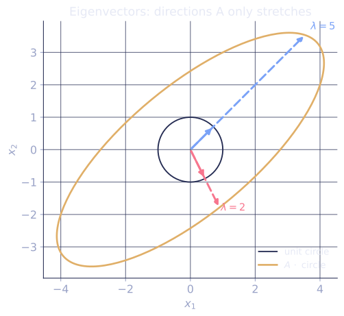
A maps the unit circle to an ellipse: a generic vector changes direction, but the two eigenvectors keep their direction and are only stretched, by λ = 5 and λ = 2.

Check it on arrays

python · numpy

import numpy as np

A = np.array([[4.0, 1.0],
              [2.0, 3.0]])

eigenvalues, eigenvectors = np.linalg.eig(A)
print("eigenvalues:", eigenvalues)       # [5, 2]
print("eigenvectors (columns):\n", eigenvectors)

# Verify: A @ v == lambda * v for each pair
for i, lam in enumerate(eigenvalues):
    v = eigenvectors[:, i]
    print(f"A@v - lam*v = {np.round(A @ v - lam * v, 10)}")  # ~zero

# Trace and det from eigenvalues
print("trace(A):", np.trace(A), "= sum of eigenvalues:", eigenvalues.sum())
print("det(A):", np.linalg.det(A), "= product of eigenvalues:", eigenvalues.prod())

# Triangular matrix: eigenvalues are the diagonal entries
T = np.array([[3.0, 5.0, 1.0],
              [0.0, 7.0, 2.0],
              [0.0, 0.0,-1.0]])
lams = np.linalg.eig(T)[0]
print("triangular eigenvalues:", np.sort(lams)[::-1], "diagonal:", [3, 7, -1])

The residuals $Av - \lambda v$ are near zero; trace and determinant match the eigenvalue sums and products.

Exercises

Exercise 1. Find the eigenvalues and a corresponding eigenvector for each, of $A = \begin{pmatrix} 2 & 1 \\ 1 & 2 \end{pmatrix}$ , working entirely by hand.

Solution

Step 1. Form the characteristic polynomial $\det(A - \lambda I) = 0$ :

\det\begin{pmatrix} 2 - \lambda & 1 \\ 1 & 2 - \lambda \end{pmatrix} = (2 - \lambda)^2 - 1 = 0.

Step 2. Expand: $(2 - \lambda)^2 = 1$ , so $2 - \lambda = \pm 1$ , giving $\lambda_1 = 1$ and $\lambda_2 = 3$ . (Check against trace and determinant: $\lambda_1 + \lambda_2 = 4 = \operatorname{tr} A$ , and $\lambda_1 \lambda_2 = 3 = \det A$ .)

Step 3. For $\lambda_1 = 1$ , solve $(A - I)v = 0$ : the rows both read $v_1 + v_2 = 0$ , so $v = (1, -1)$ . For $\lambda_2 = 3$ , solve $(A - 3I)v = 0$ : the rows read $-v_1 + v_2 = 0$ , so $v = (1, 1)$ . The two eigenvectors are orthogonal, the symmetry of $A$ foreshadowing the spectral theorem.

Exercise 2. Prove that if $\lambda$ is an eigenvalue of an invertible matrix $A$ , then $1/\lambda$ is an eigenvalue of $A^{-1}$ , with the same eigenvector.

Solution

Step 1. Start from the eigenpair relation $Av = \lambda v$ with $v \neq 0$ . Since $A$ is invertible, $\lambda \neq 0$ (a zero eigenvalue would mean a nonzero $v$ in $\ker A$ , contradicting invertibility).

Step 2. Apply $A^{-1}$ to both sides: $A^{-1} A v = A^{-1}(\lambda v)$ , i.e. $v = \lambda\, A^{-1} v$ .

Step 3. Divide by $\lambda \neq 0$ : $A^{-1} v = \tfrac{1}{\lambda} v$ . So $v$ is an eigenvector of $A^{-1}$ with eigenvalue $1/\lambda$ .

Exercise 3 (code). A real matrix can have complex eigenvalues in conjugate pairs. Build the rotation matrix $R_\theta$ for $\theta = 30^\circ$ , confirm its eigenvalues are $e^{\pm i\theta}$ , and check the trace/determinant relations hold over the complex eigenvalues.

Solution

python · numpy

import numpy as np

theta = np.deg2rad(30.0)
R = np.array([[np.cos(theta), -np.sin(theta)],
              [np.sin(theta),  np.cos(theta)]])

eigvals = np.linalg.eigvals(R)
expected = np.array([np.exp(1j * theta), np.exp(-1j * theta)])

# Eigenvalues are e^{+/- i theta} (order may differ, so compare sorted).
assert np.allclose(np.sort_complex(eigvals), np.sort_complex(expected))

# Trace = sum of eigenvalues, det = product (both real for a real matrix).
assert np.isclose(eigvals.sum().real, np.trace(R))
assert np.isclose(eigvals.prod().real, np.linalg.det(R))
print("eigenvalues:", np.round(eigvals, 4))

The eigenvalues land on the unit circle at angle $\pm\theta$ , their sum equals $\operatorname{tr} R = 2\cos\theta$ , and their product equals $\det R = 1$ : a pure rotation scales nothing.

When a symmetric matrix enters the picture, its eigenvalues are always real and its eigenvectors always orthogonal: the spectral theorem, the subject of the next lesson.

References

[1]Strang, G. (2016). Introduction to Linear Algebra (5th ed.). Wellesley-Cambridge Press. Eigenvalues, eigenvectors, and their geometric meaning.↩
[2]Horn, R. A., & Johnson, C. R. (2012). Matrix Analysis (2nd ed.). Cambridge University Press. The characteristic polynomial, trace/determinant relations, and multiplicities.↩