Random variables and distributions

A probability space tells you which outcomes are possible and how likely each event is, but outcomes are often unwieldy objects (a card, a coin face, a point in space). A random variable attaches a number to each outcome, turning probability into something we can average, plot, and compute with.

Definition

A random variable is a function $X: \Omega \to \mathbb{R}$ that assigns a real number to each outcome[1]. For a die, $X(\omega) = \omega$ is the face value; for two coins, $X$ could count the number of heads.

The probability of $X$ landing in a set $S \subseteq \mathbb{R}$ is the probability of the outcomes that map into $S$:

The right-hand side is a probability of an event in the original space; the left-hand side is the notation we actually use. The distribution of $X$ is the collection of these probabilities over all $S$.

The cumulative distribution function

The cumulative distribution function (CDF) of $X$ is[2]

It works for any random variable, discrete or continuous. Three properties follow directly from the probability axioms:

1. Monotone nondecreasing: if $x_1 \le x_2$ then $\{X \le x_1\} \subseteq \{X \le x_2\}$, so $F_X(x_1) \le F_X(x_2)$ by monotonicity of $P$.
2. Limits: $F_X(x) \to 0$ as $x \to -\infty$ and $F_X(x) \to 1$ as $x \to +\infty$.
3. Right-continuous.

Any function with these properties is the CDF of some random variable.

Discrete random variables and the PMF

$X$ is discrete if it takes values in a finite or countable set. Its distribution is captured by the probability mass function (PMF)

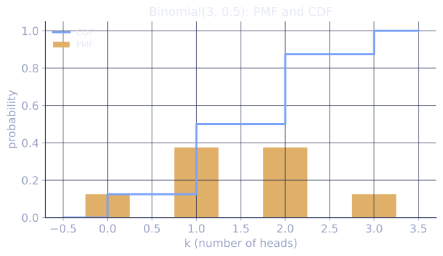
The CDF is a sum of masses: $F_X(x) = \sum_{x_i \le x} p_X(x_i)$, a staircase that jumps by $p_X(x_i)$ at each value $x_i$.

Continuous random variables and the PDF

$X$ is continuous if its CDF can be written as an integral

for some nonnegative probability density function (PDF) $f_X$. By the fundamental theorem of calculus, $f_X(x) = F_X'(x)$ where the derivative exists.

A density is not a probability: $f_X(x)$ can exceed 1. Probabilities come from integrating it over an interval,

and a single point has probability zero, $P(X = a) = 0$. The normalization is $\int_{-\infty}^\infty f_X(x)\, dx = 1$.

The density as a limit

The interpretation of $f_X$ is a probability per unit length: for a small width $\varepsilon$,

So $f_X(x)$ measures how concentrated the probability is near $x$, just as mass density measures how concentrated matter is near a point.

Check it on arrays

Sampling lets us reconstruct both the PMF (by counting) and the PDF (by a normalized histogram), and verify that the empirical CDF tracks the theoretical one.

import numpy as np

rng = np.random.default_rng(1)
N = 200_000

# Discrete: number of heads in 3 fair coin flips -> values 0..3
flips = rng.integers(0, 2, size=(N, 3))
X = flips.sum(axis=1)
values, counts = np.unique(X, return_counts=True)
pmf = counts / N
# Exact PMF: C(3,k)/8
from math import comb
exact = np.array([comb(3, k) for k in values]) / 8
for v, p, e in zip(values, pmf, exact):
    print(f"P(X={v}) = {p:.4f}   exact {e:.4f}")
print("PMF sums to:", pmf.sum())

# Continuous: standard normal, compare histogram to the PDF
Z = rng.normal(size=N)
hist, edges = np.histogram(Z, bins=50, density=True)   # density=True -> integrates to 1
centers = 0.5 * (edges[:-1] + edges[1:])
pdf = np.exp(-centers**2 / 2) / np.sqrt(2 * np.pi)
print("max |hist - pdf|:", np.max(np.abs(hist - pdf)))   # small

# Empirical CDF at 0 should be ~0.5
print("F_Z(0) empirical:", (Z <= 0).mean(), "  theoretical 0.5")

Counting recovers the binomial PMF, the normalized histogram matches the Gaussian density, and the empirical CDF lands on the theoretical value.

Exercises

Exercise 1. A discrete random variable $X$ has PMF $p_X(1) = 0.2$, $p_X(2) = 0.5$, $p_X(3) = 0.3$. Write its CDF $F_X(x)$ as a staircase and evaluate $F_X(2)$ and $P(1 < X \le 3)$.

Exercise 2. A continuous random variable has density $f_X(x) = 2x$ for $0 \le x \le 1$ and $0$ elsewhere. Confirm it is a valid density, find the CDF, and compute $P(X \le 0.5)$.

Exercise 3 (code). Sample from the density $f_X(x) = 2x$ on $[0, 1]$ by inverse transform: if $U$ is uniform on $[0, 1]$, then $X = \sqrt{U}$ has CDF $x^2$. Verify the empirical CDF at $0.5$ matches the theoretical $0.25$.

import numpy as np

rng = np.random.default_rng(4)
N = 500_000
U = rng.random(N)
X = np.sqrt(U)                      # inverse of CDF F(x) = x^2 on [0, 1]

emp_cdf_half = (X <= 0.5).mean()    # should approach F(0.5) = 0.25
theoretical = 0.5**2

assert np.isclose(emp_cdf_half, theoretical, atol=2e-3)
print("F_X(0.5) empirical:", round(emp_cdf_half, 4),
      " theoretical:", theoretical)

The next lesson collapses a whole distribution into a single representative number: its expectation.

References

- [1]Wasserman, L. (2004). All of Statistics. Springer. Ch. 2, random variables and distribution functions. doi:10.1007/978-0-387-21736-9↩
- [2]Casella, G., & Berger, R. L. (2002). Statistical Inference (2nd ed.). Duxbury. §1.5-1.6, CDFs and density/mass functions.↩