Markov, Chebyshev, and Jensen inequalities

Exact distributions are often unavailable, but a mean or a variance is. The basic probability inequalities turn those one or two numbers into guarantees: how much probability can sit far from the mean, and how a convex function reshapes an average. They are also the building blocks of the law of large numbers and of generalization bounds in learning theory.

Markov's inequality

For a nonnegative random variable $X \ge 0$ and any $a > 0$[1],

Proof. Define the indicator $\mathbf{1}[X \ge a]$, which is 1 when $X \ge a$ and 0 otherwise. Because $X \ge 0$, the pointwise bound $a\,\mathbf{1}[X \ge a] \le X$ holds: when the indicator is 1, $X \ge a$; when it is 0, the left side is 0 and $X \ge 0$. Taking expectations and using monotonicity, $a\,P(X \ge a) = \mathbb{E}[a\,\mathbf{1}[X \ge a]] \le \mathbb{E}[X]$. Divide by $a$. $\qquad\blacksquare$

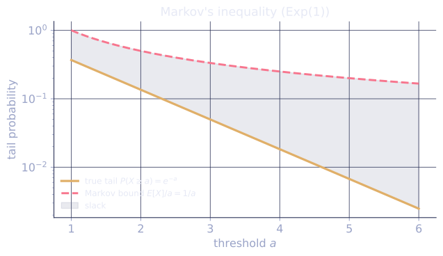
Markov uses only the mean, so the bound is weak, but it needs nothing else.

Chebyshev's inequality

Applying Markov to the nonnegative variable $(X - \mu)^2$ with threshold $k^2$ turns a variance into a two-sided tail bound. With $\mu = \mathbb{E}[X]$ and $\sigma^2 = \operatorname{Var}(X)$, for any $k > 0$:

Stated in standard-deviation units $k = c\sigma$: $P(|X - \mu| \ge c\sigma) \le 1/c^2$. At least 75% of any distribution's mass lies within two standard deviations, 89% within three, regardless of shape. This distribution-free guarantee is what powers the law of large numbers.

Jensen's inequality

For a convex function $\varphi$ (one curving upward, so every chord lies above the graph)[2],

The inequality reverses for concave $\varphi$.

Proof. Convexity gives a supporting line at the point $\mu = \mathbb{E}[X]$: there is a slope $c$ with $\varphi(x) \ge \varphi(\mu) + c(x - \mu)$ for all $x$. Take expectations of both sides. The right side becomes $\varphi(\mu) + c(\mathbb{E}[X] - \mu) = \varphi(\mu)$, since $\mathbb{E}[X] = \mu$. So $\mathbb{E}[\varphi(X)] \ge \varphi(\mu)$. $\qquad\blacksquare$

Consequences appear everywhere: $\mathbb{E}[X^2] \ge (\mathbb{E}[X])^2$ (which is just $\operatorname{Var}(X) \ge 0$), and for concave $\log$, $\mathbb{E}[\log X] \le \log \mathbb{E}[X]$, the step behind the nonnegativity of KL divergence two lessons from now.

Check it on arrays

import numpy as np

rng = np.random.default_rng(9)
N = 2_000_000

# Markov on a nonnegative variable: Exponential(rate=1), mean 1
X = rng.exponential(1.0, N)
for a in [2.0, 4.0, 6.0]:
    print(f"P(X>={a}) = {np.mean(X >= a):.4f}  Markov bound {1.0/a:.4f}")

# Chebyshev: any distribution, here a mixture
Y = np.where(rng.random(N) < 0.5, rng.normal(0, 1, N), rng.normal(0, 3, N))
mu, sigma = Y.mean(), Y.std()
for c in [2.0, 3.0]:
    emp = np.mean(np.abs(Y - mu) >= c * sigma)
    print(f"P(|Y-mu|>={c}sigma) = {emp:.4f}  Chebyshev bound {1/c**2:.4f}")

# Jensen for convex phi(x)=x^2: phi(E[X]) <= E[phi(X)]
print("phi(E[X]) =", round(X.mean()**2, 4), "<= E[phi(X)] =", round((X**2).mean(), 4))

Every empirical tail probability sits below its Markov or Chebyshev bound, and Jensen's inequality holds for the square.

Exercises

Exercise 1. A nonnegative random variable has mean $\mathbb{E}[X] = 5$. Use Markov's inequality to bound $P(X \ge 20)$, then $P(X \ge 10)$. State why the second bound is weaker as a guarantee.

Exercise 2. Show that Chebyshev's inequality gives the "at least 75% within two standard deviations" claim, and find the smallest $c$ for which Chebyshev guarantees at least 90% of the mass lies within $c$ standard deviations of the mean.

Exercise 3 (code). Pick a convex function $\varphi(x) = e^x$ and a random variable, and verify Jensen's inequality $\varphi(\mathbb{E}[X]) \le \mathbb{E}[\varphi(X)]$. Then check the gap vanishes for an affine (both convex and concave) function.

import numpy as np

rng = np.random.default_rng(0)
N = 2_000_000

X = rng.normal(0.0, 1.0, N)

# Convex phi(x) = e^x: Jensen says phi(E[X]) <= E[phi(X)]
lhs = np.exp(X.mean())
rhs = np.exp(X).mean()
print("phi(E[X]) =", round(lhs, 4), "<= E[phi(X)] =", round(rhs, 4))
assert lhs <= rhs

# Affine psi(x) = 3x + 1 is both convex and concave: Jensen holds with equality
psi = lambda x: 3 * x + 1
print("psi(E[X]) =", round(psi(X.mean()), 4),
      " E[psi(X)] =", round(psi(X).mean(), 4))
assert np.isclose(psi(X.mean()), psi(X).mean(), atol=1e-3)

These bounds make the next lesson's limit theorems precise: as samples accumulate, the average concentrates on the mean.

References

- [1]Wasserman, L. (2004). All of Statistics. Springer. §4.1, the Markov and Chebyshev inequalities. doi:10.1007/978-0-387-21736-9↩
- [2]Cover, T. M., & Thomas, J. A. (2006). Elements of Information Theory (2nd ed.). Wiley. §2.6, Jensen's inequality and its consequences. doi:10.1002/047174882X↩