Expectation and the law of the unconscious statistician

A distribution carries a lot of detail. Often the single most useful summary is its center of mass: the value the random variable takes on average over many trials. That is the expectation, and its single most useful property, linearity, holds with no independence assumptions at all.

Definition

The expectation (or mean) of a random variable $X$ is a probability-weighted average of its values[1]. For a discrete $X$ with PMF $p_X$,

and for a continuous $X$ with PDF $f_X$,

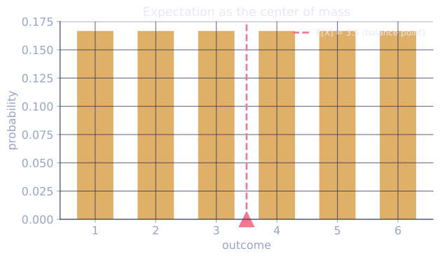
whenever the sum or integral converges absolutely. The expectation is a single number, often written $\mu$. It is the balance point of the distribution: the place where the PMF or PDF would balance on a knife edge.

The law of the unconscious statistician

To compute the expectation of $g(X)$ for some function $g$, one route is to find the distribution of the new random variable $Y = g(X)$, then average. The law of the unconscious statistician (LOTUS) says you can skip that step and weight $g(x)$ by the distribution of $X$ directly[2]:

Why it holds (discrete case). Group the outcomes by the value $y$ that $g$ takes:

The inner step replaces $y$ by $g(x)$, valid because the sum only includes $x$ with $g(x) = y$. Summing over the groups recovers a sum over all $x$.

Linearity of expectation

For any random variables $X, Y$ and constants $a, b$,

Derivation (discrete, joint PMF $p$). By LOTUS applied to the function $g(x, y) = ax + by$,

The first double sum marginalizes out $y$ to give $\sum_x x\, p_X(x) = \mathbb{E}[X]$; the second gives $\mathbb{E}[Y]$. So the expectation of a sum is the sum of expectations, with no independence assumption. This is what makes linearity so powerful: it applies even to highly dependent variables.

A worked use of linearity

How many heads in $n$ flips of a coin with $P(\text{head}) = q$? Let $X_i$ be the indicator that flip $i$ is heads, so $\mathbb{E}[X_i] = q$. The total is $X = \sum_{i=1}^n X_i$, and by linearity

with no need to touch the binomial PMF. Indicator random variables plus linearity solve a large fraction of counting-expectation problems.

Check it on arrays

import numpy as np

rng = np.random.default_rng(2)
N = 500_000

# E[X] for a die
X = rng.integers(1, 7, size=N)
print("E[die]:", X.mean(), "  exact 3.5")

# LOTUS: E[X^2] computed by weighting g(x)=x^2, no distribution of X^2 needed
print("E[X^2]:", (X**2).mean(), "  exact", sum(x**2 for x in range(1, 7)) / 6)

# Linearity without independence: Y = X, so X + Y = 2X are perfectly dependent
Y = X
print("E[X + Y]:", (X + Y).mean(), "  E[X]+E[Y]:", X.mean() + Y.mean())

# Indicators + linearity: heads in n=10 flips, q=0.3
q, n = 0.3, 10
flips = (rng.random(size=(N, n)) < q)
total = flips.sum(axis=1)
print("E[heads]:", total.mean(), "  n*q:", n * q)

The die mean lands on 3.5, LOTUS gives the right second moment, linearity holds even for the perfectly dependent pair, and the indicator sum averages to $nq$.

Exercises

Exercise 1. A fair six-sided die is rolled once. Use LOTUS to compute $\mathbb{E}[X^2]$ directly, without finding the distribution of $X^2$.

Exercise 2. Draw a card position uniformly: a hat holds $n$ cards numbered $1$ to $n$, you draw all $n$ in random order. Let $X$ be the number of cards that land in their own position (a "fixed point"). Use indicator variables and linearity to show $\mathbb{E}[X] = 1$ for every $n$.

Exercise 3 (code). Verify Exercise 2 by simulation: for several values of $n$, shuffle $1, \dots, n$ many times and confirm the average number of fixed points is close to 1.

import numpy as np

rng = np.random.default_rng(0)
trials = 500_000

for n in [3, 10, 52]:
    perms = rng.permuted(np.broadcast_to(np.arange(n), (trials, n)), axis=1)
    fixed = (perms == np.arange(n)).sum(axis=1)
    mean_fixed = fixed.mean()
    print(f"n={n:3d}  E[fixed points] = {mean_fixed:.4f}  (exact 1.0)")
    assert np.isclose(mean_fixed, 1.0, atol=0.02)

That second moment is the raw material for the next lesson, which measures spread: variance.

References

- [1]Casella, G., & Berger, R. L. (2002). Statistical Inference (2nd ed.). Duxbury. §2.2, expected values and their properties.↩
- [2]Wasserman, L. (2004). All of Statistics. Springer. Ch. 3, expectation, linearity, and the law of the unconscious statistician. doi:10.1007/978-0-387-21736-9↩