Maximum likelihood estimation

Distributions come with parameters: the rate of a Poisson, the mean of a Gaussian. Given data and a chosen distribution family, maximum likelihood picks the parameter that makes the observed data as probable as possible[1]. It is the default estimator behind logistic regression, Gaussian fits, and the cross-entropy loss of classification.

The likelihood function

Suppose the data $x_1, \dots, x_n$ are i.i.d. from a distribution with PMF or PDF $p(x \mid \theta)$. The likelihood is the probability of the data viewed as a function of the parameter[2]:

The data are fixed; $\theta$ varies. The maximum likelihood estimate (MLE) is the maximizer

Why the log

Products of many small probabilities underflow and are awkward to differentiate. Because $\log$ is strictly increasing, it does not move the maximizer, and it turns the product into a sum:

Maximize the log-likelihood $\ell$ instead. At an interior maximum its gradient vanishes:

The summand $\nabla_\theta \log p(x_i \mid \theta)$ is the score; the MLE sets the total score to zero.

Worked example: the Gaussian

For $\mathcal{N}(\mu, \sigma^2)$,

Summing and differentiating in $\mu$:

the sample mean. Differentiating in $\sigma^2$:

the (biased) sample variance with divisor $n$. The MLE recovers the natural plug-in estimators.

Properties

Under regularity conditions, the MLE is consistent (converges to the true parameter as $n \to \infty$, by the law of large numbers applied to the score), asymptotically normal, and asymptotically efficient (it achieves the smallest possible variance, set by the Fisher information of a later lesson). It can be biased at finite $n$, as $\hat\sigma^2$ shows: dividing by $n - 1$ instead removes that bias.

Check it on arrays

import numpy as np

rng = np.random.default_rng(11)
N = 100_000

# Gaussian MLE: closed form equals sample mean and (1/n) sample variance
true_mu, true_sigma = 2.0, 1.5
data = rng.normal(true_mu, true_sigma, N)
mu_hat = data.mean()
sigma2_hat = ((data - mu_hat)**2).mean()    # divisor n (MLE)
print("mu_hat:", round(mu_hat, 4), "  true", true_mu)
print("sigma_hat:", round(np.sqrt(sigma2_hat), 4), "  true", true_sigma)

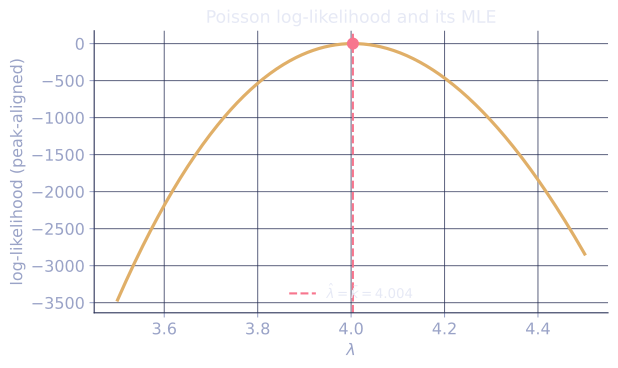
# Poisson MLE for lambda is the sample mean: maximize sum(x log L - L)
true_lam = 4.0
counts = rng.poisson(true_lam, N)
lam_hat = counts.mean()
print("lambda_hat:", round(lam_hat, 4), "  true", true_lam)

# Verify by a grid search on the log-likelihood
grid = np.linspace(3.5, 4.5, 2001)
# sum over data of (x log lam - lam), constant log(x!) dropped
ll = counts.sum() * np.log(grid) - N * grid
print("grid argmax:", round(grid[np.argmax(ll)], 4))

The closed-form Gaussian and Poisson estimators recover the true parameters, and the grid search confirms the Poisson MLE is the sample mean.

Exercises

Exercise 1. A coin lands heads $h$ times in $n$ independent flips, with unknown head probability $\theta$. Derive the MLE $\hat\theta$ by maximizing the log-likelihood.

Exercise 2. For data $x_1, \dots, x_n$ i.i.d. Exponential with rate $\lambda$ (density $p(x \mid \lambda) = \lambda e^{-\lambda x}$ for $x \ge 0$), derive $\hat\lambda$.

Exercise 3 (code). Generate $n = 200{,}000$ Exponential samples with true rate $\lambda = 3$. Verify that the closed-form MLE $1/\bar x$ from Exercise 2 matches the maximizer of the log-likelihood found by a grid search.

import numpy as np

rng = np.random.default_rng(7)
N = 200_000
true_lam = 3.0
x = rng.exponential(scale=1 / true_lam, size=N)   # numpy scale = 1/rate

lam_closed = 1 / x.mean()                          # MLE from Exercise 2

# Grid search on the log-likelihood ell(lam) = N log(lam) - lam * sum(x)
grid = np.linspace(2.5, 3.5, 4001)
ll = N * np.log(grid) - grid * x.sum()
lam_grid = grid[np.argmax(ll)]

assert np.isclose(lam_closed, lam_grid, atol=1e-3)
print("closed form:", round(lam_closed, 4), " grid:", round(lam_grid, 4))

The next lesson adds a prior on top of the likelihood, turning estimation into Bayesian inference.

References

- [1]Casella, G., & Berger, R. L. (2002). Statistical Inference (2nd ed.). Duxbury. §7.2, maximum likelihood estimators and their derivation.↩
- [2]Wasserman, L. (2004). All of Statistics. Springer. Ch. 9, the likelihood function and MLE. doi:10.1007/978-0-387-21736-9↩