Newton's method

Gradient descent uses only the slope and so cannot tell a gently curving valley from a sharp one. Newton's method uses the curvature too: it fits a quadratic to the function and jumps to that quadratic's minimum. Near a solution it converges quadratically, doubling the number of correct digits each step, which makes it the template for second-order optimization.

Derivation from a quadratic model

Approximate $f$ near $x_t$ by its second-order Taylor expansion:

This is a quadratic in $x$. Setting its gradient to zero, $\nabla \hat f(x) = \nabla f(x_t) + \nabla^2 f(x_t)(x - x_t) = 0$, and solving for $x$ gives the Newton step:

Where gradient descent uses a scalar step $\eta$, Newton uses the inverse Hessian as a matrix-valued step that rescales and rotates the gradient to match the local curvature. On a quadratic objective, the model is exact and Newton reaches the minimum in a single step.

Affine invariance

Newton's method is affine invariant: applying a linear change of variables $x = Ay$ produces the same sequence of iterates (mapped through $A$). The condition number that crippled gradient descent does not affect Newton, because the inverse Hessian undoes the coordinate scaling. There is no learning rate to tune for conditioning.

Quadratic convergence

Near a minimizer $x^\star$ where the Hessian is positive definite and Lipschitz, the Newton error obeys

Once the error is small, squaring it each step means the count of accurate digits roughly doubles per iteration. This quadratic rate is far faster than the linear rate of gradient descent, but it is local: it holds only once the iterate is close enough that the quadratic model is trustworthy.

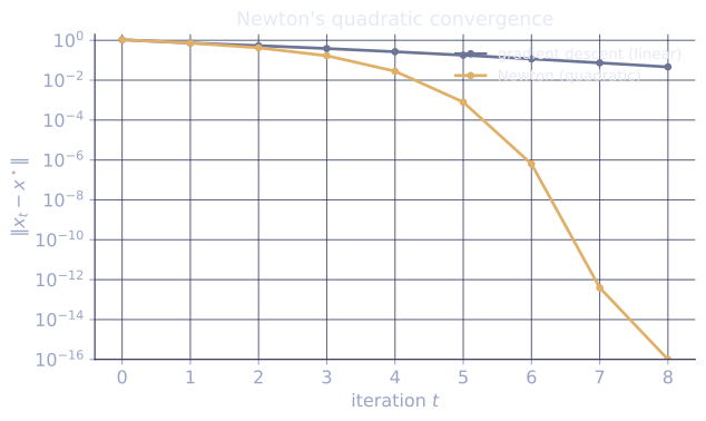
To see "doubling digits" as real numbers, run the closing block's example ($f(x) = \sum_i (x_i - \log x_i)$, minimized at the all-ones point). Once the iterate enters the basin, the error norm and its accurate-digit count ($-\log_{10}$ error) fall as:

• step 4: error $\approx 2.8 \times 10^{-2}$, about $1.6$ digits.
• step 5: error $\approx 7.9 \times 10^{-4}$, about $3.1$ digits.
• step 6: error $\approx 6.3 \times 10^{-7}$, about $6.2$ digits.

Each step nearly doubles the digit count ($1.6 \to 3.1 \to 6.2$), the signature of a quadratic rate. The contrast is sharp against gradient descent on the identical problem from the identical start: with $\eta = 0.4$ it decays linearly and still sits at error $\approx 1.2 \times 10^{-1}$ at step 6, where Newton has reached $10^{-7}$. Same function, same starting point; the curvature information is the whole difference.

Practical cautions

Two issues keep raw Newton from being used directly on large problems:

• Cost. Forming and inverting the $n \times n$ Hessian is $O(n^3)$ per step, infeasible when $n$ is in the millions. Solving $\nabla^2 f\, p = -\nabla f$ rather than inverting, and quasi-Newton approximations (next lesson), address this.
• Non-convexity. If the Hessian is not positive definite, the Newton step can point uphill or toward a saddle. Damped Newton (a line search on the step) and trust-region or Hessian-modification methods restore a descent guarantee far from the optimum.

Check it on arrays

import numpy as np

# Strongly convex, non-quadratic: f(x) = sum(x_i - log x_i) on x > 0, min at all-ones.
# grad = 1 - 1/x, Hessian = diag(1/x^2). Newton converges globally on (0, 2).
f = lambda x: np.sum(x - np.log(x))
grad = lambda x: 1 - 1 / x
hess = lambda x: np.diag(1 / x**2)
opt = np.ones(3)

x_n = np.array([1.5, 0.5, 1.8])                  # inside the Newton basin (0, 2)
x_g = x_n.copy()

print("step |  Newton err     |  GD err (eta=0.4)")
for t in range(8):
    print(f"{t:>4} | {np.linalg.norm(x_n - opt):.2e}      | {np.linalg.norm(x_g - opt):.2e}")
    x_n = x_n - np.linalg.solve(hess(x_n), grad(x_n))
    x_g = x_g - 0.4 * grad(x_g)                   # gradient descent for contrast

print("Newton final error:", f"{np.linalg.norm(x_n - opt):.2e}")

# Single-step exactness on a quadratic: f = 0.5 x^T A x - b^T x
A = np.array([[3.0, 1.0], [1.0, 2.0]]); b = np.array([1.0, -1.0])
x = np.array([9.0, -4.0])
x = x - np.linalg.solve(A, A @ x - b)            # one Newton step
print("one Newton step error:", np.linalg.norm(x - np.linalg.solve(A, b)))

Newton's error collapses quadratically while gradient descent decays linearly, and a single Newton step solves the quadratic exactly.

Exercises

Exercise 1. Take the quadratic $f(x) = \tfrac12 x^\top A x - b^\top x$ with $A = \left(\begin{smallmatrix} 3 & 1 \\ 1 & 2 \end{smallmatrix}\right)$ and $b = \left(\begin{smallmatrix} 1 \\ -1 \end{smallmatrix}\right)$. Starting from any $x_0$, compute the Newton step by hand and show it lands on the exact minimizer in one move.

Exercise 2. Newton's method is affine invariant. Take the one-dimensional change of variables $x = a y$ with constant $a \ne 0$, define $h(y) = f(ay)$, and show that one Newton step on $h$ in $y$ maps through $a$ to the same Newton step on $f$ in $x$.

Exercise 3 (code). For the scalar root-finding view, Newton on $f'(x) = x^2 - 2$ (i.e. minimizing an antiderivative whose stationary point is $\sqrt 2$) is $x_{t+1} = x_t - (x_t^2 - 2)/(2 x_t)$. Starting at $x_0 = 2$, iterate and confirm the quadratic doubling of accurate digits by checking that the error at each step is bounded by the square of the previous error times a constant.

import numpy as np

root = np.sqrt(2.0)
x = 2.0
errs = []
for _ in range(6):
    errs.append(abs(x - root))
    x = x - (x**2 - 2.0) / (2.0 * x)
errs = np.array(errs)

# Quadratic convergence: e_{t+1} <= C e_t^2. The Newton constant here is 1/(2 root).
C = 1.0 / (2.0 * root)
ratios = errs[1:] / errs[:-1]**2          # should stay near or below C
print("errors:", errs)
print("e_{t+1}/e_t^2:", ratios)

assert np.all(ratios[:-1] <= C + 1e-9)    # bound holds (last entry is ~0/0 noise)
assert errs[3] < 1e-3                      # already deep in the basin by step 3
print("converged to:", x)

The next lesson approximates the Hessian from gradients to keep this speed without the $O(n^3)$ cost.

References

- [1]Nocedal, J., & Wright, S. J. (2006). Numerical Optimization (2nd ed.), §3.3. Springer. The Newton step and its derivation from the quadratic model (doi:10.1007/978-0-387-40065-5).↩
- [2]Boyd, S., & Vandenberghe, L. (2004). Convex Optimization, §9.5. Cambridge University Press. Affine invariance and the local quadratic convergence of Newton's method.↩