Bayesian optimization

Some objectives have no gradient and cost a fortune to evaluate: a hyperparameter setting that takes hours to train, a physical experiment, a chemical assay. Bayesian optimization spends computation to be sample-efficient. It fits a probabilistic model of the objective, then uses that model's uncertainty to choose the single most informative point to try next.

The setting

Minimize (or maximize) $f(x)$ where each evaluation is expensive and no derivatives are available. The budget is a few dozen evaluations, not millions, so the goal is to find a good $x$ in as few queries as possible. Two ingredients make this work: a surrogate model that predicts $f$ with calibrated uncertainty, and an acquisition function that turns those predictions into the next query.

The Gaussian-process surrogate

A Gaussian process (GP) models the unknown function as a distribution over functions, specified by a covariance kernel $k(x, x')$ that says how correlated the values at two inputs are. The common choice is the RBF kernel

which makes nearby inputs strongly correlated and distant ones independent, with length scale $\ell$. Given observations $(X, \mathbf{y})$, the GP posterior at a new point $x_\star$ is Gaussian with closed-form mean and variance:

where $K_{ij} = k(x_i, x_j)$, $(k_\star)_i = k(x_i, x_\star)$, and $\sigma_n^2$ is observation noise[1]. The mean is the prediction; the variance grows away from observed points, encoding "I have not looked here yet". This is the conjugate Gaussian update of the MAP lesson, lifted to functions.

The acquisition function

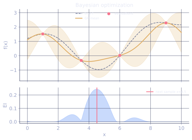
The acquisition function scores each candidate by how worthwhile it is to evaluate, balancing exploitation (low predicted mean) against exploration (high variance). Expected improvement (EI), for minimizing with current best $f^\star = \min y_i$, is the expected amount by which a query at $x$ would beat the best so far:

with $\Phi, \phi$ the standard normal CDF and PDF. EI is large where the mean is low (promising) or the variance is high (uncertain), and it is zero where the model is confident the value is worse than $f^\star$. The next query is $\arg\max_x \text{EI}(x)$[2].

The two terms encode exploitation and exploration, and a few computed values make their tug-of-war concrete. Take the current best $f^\star = 0$:

• Exploration, isolated. A point predicted above the best, $\mu = 0.5$, looks unpromising on its mean alone. With small uncertainty $s = 0.1$ its EI is $0$: the model is sure it is worse, nothing to gain. Widen the uncertainty to $s = 1.0$ at the same mean and EI rises to $\approx 0.198$, because now the upside tail might beat $f^\star$. Same predicted mean, opposite verdicts; the variance term is the whole difference.
• Exploitation, isolated. A point predicted below the best, $\mu = -0.5$ with $s = 0.1$, has EI $\approx 0.5$, essentially its mean improvement: the gain is locked in, not speculative.
• Ruled out. A point with $\mu = 2.0$ and tiny $s = 0.05$ has EI $\approx 0$ (under $10^{-5}$): far above the best and almost certain, so no query is worth spending there.

This is the named confusion behind "explore vs exploit": EI does not optimize the predicted mean, and it does not chase raw uncertainty either. It scores the expected improvement over the current best, which is why a high-variance point that looks mediocre on its mean can outrank a confident, slightly-better one.

The loop

1. Fit the GP to all evaluations so far.
2. Maximize the acquisition function to pick the next $x$.
3. Evaluate the true (expensive) $f$ there, add the point, repeat.

Each step uses cheap GP and acquisition computation to decide where to spend one expensive evaluation, which is why it dominates random or grid search for hyperparameter tuning.

Check it on arrays

import numpy as np
import math

rng = np.random.default_rng(0)

# Expensive black box (here cheap, for demonstration): minimize on [0, 10].
f = lambda x: np.sin(x) + 0.3 * (x - 4)**2 / 4

def rbf(a, b, ell=1.0, sf=1.0):
    d2 = (a[:, None] - b[None, :])**2
    return sf**2 * np.exp(-d2 / (2 * ell**2))

_erf = np.vectorize(math.erf)
normal_cdf = lambda z: 0.5 * (1 + _erf(np.asarray(z, float) / np.sqrt(2)))
normal_pdf = lambda z: np.exp(-z**2 / 2) / np.sqrt(2 * np.pi)

cand = np.linspace(0, 10, 400)              # candidate grid for the acquisition max
X = np.array([1.0, 9.0])                    # two initial evaluations
y = f(X)
noise = 1e-2                                # nugget keeps the kernel matrix well-conditioned

for step in range(12):
    K = rbf(X, X) + noise * np.eye(len(X))
    alpha = np.linalg.solve(K, y)           # solve, never form the inverse
    ks = rbf(X, cand)
    mu = ks.T @ alpha
    var = np.maximum(rbf(cand, cand).diagonal() - np.sum(ks * np.linalg.solve(K, ks), axis=0), 1e-12)
    s = np.sqrt(var)
    f_best = y.min()
    z = (f_best - mu) / s
    ei = (f_best - mu) * normal_cdf(z) + s * normal_pdf(z)
    idx = np.argmax(ei)
    X = np.append(X, cand[idx])
    y = np.append(y, f(cand[idx]))
    cand = np.delete(cand, idx)             # do not re-query the same point

best = X[np.argmin(y)]
# True minimum by dense search for reference
dense = np.linspace(0, 10, 100_000)
print("BO best x:", round(best, 3), " f:", round(f(best), 4))
print("true  best x:", round(dense[np.argmin(f(dense))], 3),
      " f:", round(f(dense).min(), 4))
print("evaluations used:", len(X))

Bayesian optimization locates the minimum to within grid resolution using only about a dozen evaluations, guided by expected improvement.

Exercises

Exercise 1. With current best $f^\star = 0$, compute the expected improvement at a candidate with posterior mean $\mu = -0.5$ and standard deviation $s = 0.1$. Use $\Phi(5) \approx 1$ and $\phi(5) \approx 1.5 \times 10^{-6}$. Confirm the lesson's claim that EI here is essentially the mean improvement.

Exercise 2. Take two candidates with the same posterior mean $\mu = 0.5$ (above the best $f^\star = 0$, so unpromising on the mean) but different uncertainties $s = 0.1$ and $s = 1.0$. Argue from the EI formula why the high-uncertainty point is preferred.

Exercise 3 (code). Implement the EI formula and verify both hand results: $\text{EI} \approx 0.5$ at $(\mu, s) = (-0.5, 0.1)$, and that the $s = 1.0$ point at $\mu = 0.5$ has strictly larger EI than the $s = 0.1$ point at the same mean.

import numpy as np
import math

_erf = np.vectorize(math.erf)
Phi = lambda z: 0.5 * (1 + _erf(np.asarray(z, float) / np.sqrt(2)))
phi = lambda z: np.exp(-np.asarray(z, float)**2 / 2) / np.sqrt(2 * np.pi)

def ei(mu, s, f_best=0.0):
    z = (f_best - mu) / s
    return (f_best - mu) * Phi(z) + s * phi(z)

ei_exploit = ei(-0.5, 0.1)            # confident improvement
ei_narrow = ei(0.5, 0.1)             # unpromising, certain
ei_wide = ei(0.5, 1.0)              # unpromising mean, uncertain

assert np.isclose(ei_exploit, 0.5, atol=1e-3)
assert ei_wide > ei_narrow
print("EI(-0.5, 0.1):", round(float(ei_exploit), 4))
print("EI(0.5, 0.1):", round(float(ei_narrow), 6),
      " EI(0.5, 1.0):", round(float(ei_wide), 4))

This closes the A3 optimization track; the next subsection, A4, examines the finite-precision arithmetic these algorithms actually run in.

References

- [1]Rasmussen, C. E., & Williams, C. K. I. (2006). Gaussian Processes for Machine Learning, §2.2. MIT Press. The GP posterior mean and variance for regression.↩
- [2]Frazier, P. I. (2018). "A tutorial on Bayesian optimization". Acquisition functions and expected improvement (arXiv:1807.02811).↩