Constrained optimization and Lagrange multipliers

Real problems come with constraints: minimize loss subject to a budget, a norm bound, or a physical law. Lagrange multipliers convert a constrained problem into an unconstrained stationarity condition by encoding each constraint with its own variable. The geometry behind it, gradients lining up at the optimum, is the seed of duality and the KKT conditions.

The problem

An equality-constrained problem is

The feasible set is the intersection of the constraint surfaces $\{x : h_i(x) = 0\}$. A solution must minimize $f$ while staying on this set; the unconstrained condition $\nabla f = 0$ no longer applies, because moving off the surface is not allowed.

The geometric condition

At a constrained minimum $x^\star$, you cannot decrease $f$ by any feasible move. A feasible move is one tangent to the constraint surface, that is, orthogonal to every constraint gradient $\nabla h_i(x^\star)$. For no such move to decrease $f$, the objective gradient must have no component along the surface: $\nabla f(x^\star)$ must lie entirely in the span of the constraint gradients.

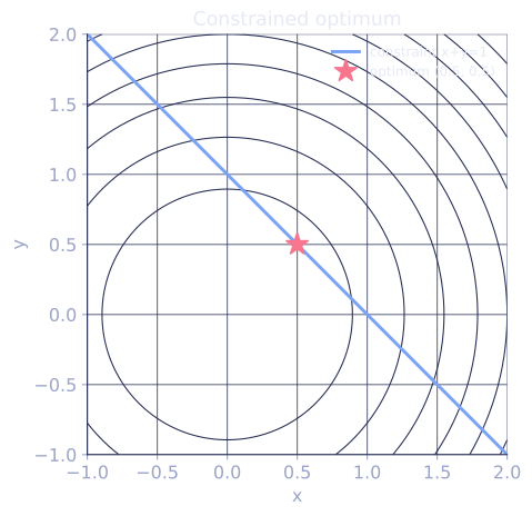
for some scalars $\lambda_i$, the Lagrange multipliers. With one constraint, this says $\nabla f$ and $\nabla h$ are parallel: the level set of $f$ is tangent to the constraint surface at the optimum. If they were not parallel, you could slide along the surface to a lower level set.

The Lagrangian

Package the condition into a single function, the Lagrangian:

Its stationarity conditions reproduce the problem exactly. Setting $\nabla_x \mathcal{L} = 0$ gives the gradient-alignment condition $\nabla f = \sum_i \lambda_i \nabla h_i$, and setting $\partial \mathcal{L}/\partial \lambda_i = 0$ gives back the constraint $h_i(x) = 0$. A constrained problem in $n$ variables becomes an unconstrained stationarity problem in $n + m$ variables $(x, \lambda)$.

What the multiplier means

The multiplier $\lambda_i$ is the sensitivity of the optimal value to the constraint. If the constraint is relaxed to $h_i(x) = c$, then

the shadow price: how much the optimum improves per unit of loosening. A zero multiplier means the constraint is not binding the objective. This economic reading carries directly into the dual variables of the next lesson.

Worked example

Minimize $f(x, y) = x^2 + y^2$ subject to $x + y = 1$. The Lagrangian is $\mathcal{L} = x^2 + y^2 - \lambda(x + y - 1)$. Stationarity: $2x - \lambda = 0$, $2y - \lambda = 0$, $x + y = 1$. The first two give $x = y$, the constraint gives $x = y = 1/2$, and $\lambda = 1$. The closest point on the line to the origin is its foot of perpendicular, confirming the gradient-alignment geometry.

Check it on arrays

import numpy as np

# min x^2 + y^2 s.t. x + y = 1, solved via the KKT linear system.
# Stationarity + constraint:  [2 0 -1][x]   [0]
#                             [0 2 -1][y] = [0]
#                             [1 1  0][lam]  [1]
M = np.array([[2.0, 0.0, -1.0],
              [0.0, 2.0, -1.0],
              [1.0, 1.0,  0.0]])
rhs = np.array([0.0, 0.0, 1.0])
x, y, lam = np.linalg.solve(M, rhs)
print(f"x={x:.4f}, y={y:.4f}, lambda={lam:.4f}")   # 0.5, 0.5, 1.0

# Shadow price: relax constraint to x + y = 1 + c, optimum f* = (1+c)^2 / 2
# df*/dc at c=0 should equal lambda
c = 1e-5
f_star = lambda cc: (1 + cc)**2 / 2
print("df*/dc:", round((f_star(c) - f_star(-c)) / (2 * c), 4), " lambda:", round(lam, 4))

# Confirm gradient alignment: grad f = lambda * grad h at the optimum
grad_f = np.array([2 * x, 2 * y])
grad_h = np.array([1.0, 1.0])
print("grad f == lambda grad h:", np.allclose(grad_f, lam * grad_h))

Solving the Lagrange system lands on $(1/2, 1/2)$ with multiplier 1, the shadow price matches the multiplier, and the objective and constraint gradients align.

Exercises

Exercise 1. Minimize $f(x, y) = x^2 + 4y^2$ subject to $x + y = 3$ using a Lagrangian. Find $x^\star, y^\star$, and the multiplier $\lambda$.

Exercise 2. Verify the shadow-price interpretation for Exercise 1 directly. Relax the constraint to $x + y = 3 + c$, find the optimal value $f^\star(c)$ as a function of $c$, and confirm $\frac{d f^\star}{dc}\big|_{c=0} = \lambda$.

Exercise 3 (code). Solve Exercise 1 by assembling and solving the KKT linear system, then verify the shadow price numerically with a central difference. Every result must match the hand answers ($x = 2.4$, $y = 0.6$, $\lambda = 4.8$).

import numpy as np

# min x^2 + 4y^2 s.t. x + y = 3, KKT system:
#  2x        - lam = 0
#         8y - lam = 0
#  x +  y          = 3
M = np.array([[2.0, 0.0, -1.0],
              [0.0, 8.0, -1.0],
              [1.0, 1.0,  0.0]])
rhs = np.array([0.0, 0.0, 3.0])
x, y, lam = np.linalg.solve(M, rhs)

assert np.allclose([x, y, lam], [2.4, 0.6, 4.8])

# Shadow price by central difference of f*(c) = 4(3+c)^2 / 5
f_star = lambda c: 4 * (3 + c)**2 / 5
c = 1e-5
slope = (f_star(c) - f_star(-c)) / (2 * c)
assert np.isclose(slope, lam, atol=1e-4)
print(f"x={x}, y={y}, lambda={lam}, df*/dc={slope:.4f}")

The next lesson generalizes the Lagrangian into a dual problem with its own optimization.

References

- [1]Bertsekas, D. P. (1999). Nonlinear Programming (2nd ed.), §3.1. Athena Scientific. The Lagrange multiplier theorem for equality-constrained problems.↩
- [2]Boyd, S., & Vandenberghe, L. (2004). Convex Optimization, §5.6. Cambridge University Press. The sensitivity (shadow-price) interpretation of the multipliers.↩