The KKT conditions

The Karush-Kuhn-Tucker (KKT) conditions are the inequality-constrained generalization of "set the gradient to zero". They are necessary at any optimum of a constrained problem with strong duality, and for convex problems they are also sufficient, turning optimization into solving a system of equations and inequalities. They characterize the solution of every SVM and convex program.

The four conditions

For the problem $\min_x f(x)$ subject to $g_i(x) \le 0$ and $h_j(x) = 0$, a point $x^\star$ with multipliers $(\lambda^\star, \nu^\star)$ satisfies the KKT conditions if:

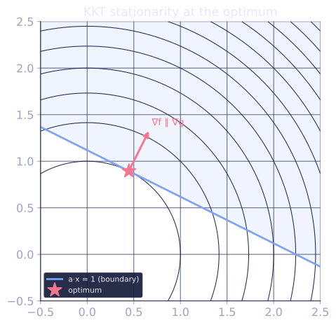
1. Stationarity. The Lagrangian gradient vanishes: $$\nabla f(x^\star) + \sum_i \lambda_i^\star \nabla g_i(x^\star) + \sum_j \nu_j^\star \nabla h_j(x^\star) = 0.$$
2. Primal feasibility. $g_i(x^\star) \le 0$ and $h_j(x^\star) = 0$.
3. Dual feasibility. $\lambda_i^\star \ge 0$ for all inequality multipliers.
4. Complementary slackness. $\lambda_i^\star\, g_i(x^\star) = 0$ for each $i$[1].

Complementary slackness

The fourth condition is the new ingredient. For each inequality, either the constraint is active ($g_i(x^\star) = 0$, the optimum sits on its boundary) or its multiplier is zero ($\lambda_i^\star = 0$, the constraint does not push). A constraint cannot simultaneously be slack ($g_i < 0$) and exert force ($\lambda_i > 0$).

Why it holds (under strong duality). At the optimum $f(x^\star) = \mathcal{D}(\lambda^\star, \nu^\star)$. Tracing the weak-duality proof with equalities, the slack terms $\sum_i \lambda_i^\star g_i(x^\star)$ must vanish; since each term is $\le 0$ (product of $\lambda_i \ge 0$ and $g_i \le 0$), each must be exactly zero. The active set, the constraints with $g_i = 0$, is what determines the solution.

Sufficiency for convex problems

For a convex problem (convex $f$ and $g_i$, affine $h_j$), the KKT conditions are not only necessary but sufficient: any point satisfying all four is a global optimum[2].

Why. Stationarity makes $x^\star$ a minimizer of the convex Lagrangian $\mathcal{L}(\cdot, \lambda^\star, \nu^\star)$. Then for any feasible $x$, $f(x) \ge \mathcal{L}(x, \lambda^\star, \nu^\star) \ge \mathcal{L}(x^\star, \lambda^\star, \nu^\star) = f(x^\star)$, where the last equality uses complementary slackness. So solving the KKT system is solving the problem.

Worked example

Minimize $f(x) = \tfrac{1}{2}\lVert x \rVert^2$ subject to $a^\top x \ge 1$, written $g(x) = 1 - a^\top x \le 0$. Stationarity: $x - \lambda a = 0$, so $x = \lambda a$. If the constraint is active, $a^\top x = 1$ gives $\lambda \lVert a\rVert^2 = 1$, so $\lambda = 1/\lVert a\rVert^2 \ge 0$ (dual feasible) and $x^\star = a/\lVert a\rVert^2$. Complementary slackness holds since $g = 0$. All four conditions check out, certifying the global optimum.

Check it on arrays

import numpy as np

# min 0.5 ||x||^2 s.t. a^T x >= 1  ->  g(x) = 1 - a^T x <= 0
a = np.array([1.0, 2.0, 2.0])
norm2 = a @ a

lam = 1.0 / norm2                                # candidate multiplier
x = lam * a                                      # from stationarity x = lam a

# Verify all four KKT conditions
stationarity = np.allclose(x - lam * a, 0)
primal_feasible = (1 - a @ x) <= 1e-9
dual_feasible = lam >= 0
slackness = np.isclose(lam * (1 - a @ x), 0)
print("stationarity:        ", stationarity)
print("primal feasibility:  ", primal_feasible)
print("dual feasibility:    ", dual_feasible)
print("compl. slackness:    ", slackness)
print("x* =", np.round(x, 4), " f* =", round(0.5 * x @ x, 4))

# Inactive-constraint case: a^T x >= -1 is already satisfied at x=0, so lam=0.
# Then x* = 0 and the constraint is slack (g < 0) with zero multiplier.
print("\ninactive constraint: x*=0, lam=0, slackness:",
      np.isclose(0.0 * (-1 - a @ np.zeros(3)), 0))

All four KKT conditions hold at the certified optimum, and the inactive-constraint case shows complementary slackness with a zero multiplier.

Exercises

Exercise 1. Solve $\min_x \tfrac12\lVert x\rVert^2$ subject to $a^\top x \ge 1$ with $a = (3, 4)$ by hand, using the KKT conditions. Report $x^\star$, $\lambda^\star$, and $f(x^\star)$.

Exercise 2. Using complementary slackness, prove that if the constraint $g(x) \le 0$ is strictly slack at the optimum ($g(x^\star) < 0$), then its multiplier must be zero, and conversely a nonzero multiplier forces the constraint active.

Exercise 3 (code). A box-constrained least squares: minimize $f(x) = \tfrac12\lVert x - c\rVert^2$ subject to $x \le u$ componentwise, with $c = (2, -1, 3)$ and $u = (1, 1, 1)$. The KKT-optimal solution clips each coordinate at its upper bound, $x^\star_i = \min(c_i, u_i)$. Verify the four KKT conditions hold at this clipped point.

import numpy as np

c = np.array([2.0, -1.0, 3.0])
u = np.array([1.0, 1.0, 1.0])

# Constraints g_i(x) = x_i - u_i <= 0. Gradient of f is x - c.
# KKT solution clips at the bound where c_i > u_i.
x = np.minimum(c, u)
lam = np.maximum(c - u, 0.0)     # multiplier active where the bound binds

g = x - u
stationarity = np.allclose((x - c) + lam, 0)   # grad f + sum lam_i grad g_i = 0
primal_feasible = np.all(g <= 1e-12)
dual_feasible = np.all(lam >= 0)
slackness = np.allclose(lam * g, 0)

assert stationarity and primal_feasible and dual_feasible and slackness
print("x* =", x, " lambda =", lam)
print("all four KKT conditions hold:",
      stationarity and primal_feasible and dual_feasible and slackness)

The next lesson returns to unconstrained methods but uses curvature: Newton's method.

References

- [1]Boyd, S., & Vandenberghe, L. (2004). Convex Optimization, §5.5. Cambridge University Press. The KKT conditions and complementary slackness.↩
- [2]Bertsekas, D. P. (1999). Nonlinear Programming (2nd ed.), §3.3. Athena Scientific. Necessity and, for convex problems, sufficiency of the KKT conditions.↩