Momentum and Nesterov acceleration

Add momentum to gradient descent and see why acceleration improves the convergence rate.

⏱ 32 minPrerequisites:Smoothness, strong convexity, and convergence rates

Gradient descent on an ill-conditioned problem zig-zags: it bounces across the steep directions while crawling along the flat ones. Momentum averages successive gradients so the consistent flat-direction signal accumulates while the oscillating steep-direction noise cancels. Nesterov's variant tunes this into a provably faster rate.

Heavy-ball momentum

Momentum (Polyak's heavy ball) maintains a velocity vector $v$ that accumulates past gradients with a decay $\beta \in [0, 1)$ :

v_{t+1} = \beta v_t + \nabla f(x_t), \qquad x_{t+1} = x_t - \eta\, v_{t+1}.

[1]

The velocity is an exponentially weighted sum of gradients: $v_{t+1} = \sum_{k=0}^{t}\beta^{t-k}\nabla f(x_k)$ . A heavy ball rolling downhill keeps moving in a consistent direction and is not deflected by every local wiggle, which is the physical picture $\beta$ controls.

Why it helps: the zig-zag cancels

On a quadratic with a steep direction (curvature $L$ ) and a flat direction (curvature $\mu$ ), plain gradient descent overshoots the steep axis and reverses sign each step, producing oscillation, while inching along the flat axis. Momentum averages those sign-flipping steep-direction gradients toward zero, while the flat-direction gradients all point the same way and build up. The effective step grows along the direction that matters and shrinks along the direction that oscillates.

Nesterov accelerated gradient

Nesterov's method evaluates the gradient at a look-ahead point, after the momentum step has been tentatively applied:

v_{t+1} = \beta v_t + \nabla f(x_t - \eta\beta v_t), \qquad x_{t+1} = x_t - \eta\, v_{t+1}.

Computing the gradient where momentum is about to land, rather than where it currently sits, lets the method correct an overshoot before committing to it. This look-ahead is what turns heuristic speedup into a provable one.

The accelerated rate

For $\mu$ -strongly convex, $L$ -smooth $f$ with condition number $\kappa = L/\mu$ , gradient descent needs $O(\kappa\log\frac{1}{\varepsilon})$ iterations. Nesterov's method, with $\beta = \frac{\sqrt\kappa - 1}{\sqrt\kappa + 1}$ , achieves

f(x_t) - f(x^\star) \le O\!\left(\Big(1 - \frac{1}{\sqrt\kappa}\Big)^t\right),

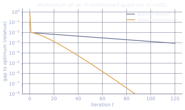
needing only $O(\sqrt\kappa\log\frac{1}{\varepsilon})$ iterations. The dependence on the condition number drops from $\kappa$ to $\sqrt\kappa$ , a large gain on ill-conditioned problems. This $\sqrt\kappa$ rate is optimal among methods that only use gradients: no first-order method can do better in the worst case[2].

On an ill-conditioned quadratic (κ = 100), Nesterov momentum drives the gap to the optimum down far faster than plain gradient descent: the √κ acceleration of the convergence rate.

Check it on arrays

python · numpy

import numpy as np

# Ill-conditioned quadratic: f(x) = 0.5 x^T A x, A = diag(mu, L)
mu, L = 1.0, 100.0
A = np.diag([mu, L])
grad = lambda x: A @ x
f = lambda x: 0.5 * x @ A @ x                    # f(x*) = 0
eta = 1.0 / L
kappa = L / mu

def gd(steps):
    x = np.array([1.0, 1.0]); gaps = []
    for _ in range(steps):
        gaps.append(f(x)); x = x - eta * grad(x)
    return np.array(gaps)

def nesterov(steps):
    beta = (np.sqrt(kappa) - 1) / (np.sqrt(kappa) + 1)
    x = np.array([1.0, 1.0]); v = np.zeros(2); gaps = []
    for _ in range(steps):
        gaps.append(f(x))
        v = beta * v + grad(x - eta * beta * v)
        x = x - eta * v
    return np.array(gaps)

g_gd, g_nag = gd(400), nesterov(400)
# Iterations to reach gap < 1e-6
def first_below(g, tol=1e-6):
    idx = np.where(g < tol)[0]
    return idx[0] if len(idx) else len(g)
print("GD steps to 1e-6:      ", first_below(g_gd))
print("Nesterov steps to 1e-6:", first_below(g_nag))
print("sqrt(kappa) =", round(np.sqrt(kappa), 1), " kappa =", kappa)

Nesterov reaches the tolerance in far fewer steps than plain gradient descent, with the gap closing on the $\sqrt\kappa$ timescale rather than $\kappa$ .

Exercises

Exercise 1. Show that the heavy-ball velocity unrolls into the exponentially weighted sum $v_{t+1} = \sum_{k=0}^{t} \beta^{t-k} \nabla f(x_k)$ , starting from $v_0 = 0$ .

Solution

Step 1. The recurrence is $v_{t+1} = \beta v_t + \nabla f(x_t)$ with $v_0 = 0$ . Compute the first few terms. With $v_0 = 0$ :

v_1 = \nabla f(x_0), \qquad v_2 = \beta\,\nabla f(x_0) + \nabla f(x_1).

Step 2. Then $v_3 = \beta v_2 + \nabla f(x_2) = \beta^2 \nabla f(x_0) + \beta\,\nabla f(x_1) + \nabla f(x_2)$ . The gradient from step $k$ has been multiplied by $\beta$ once per later step.

Step 3. Induction: assume $v_{t} = \sum_{k=0}^{t-1}\beta^{t-1-k}\nabla f(x_k)$ . Then

v_{t+1} = \beta v_t + \nabla f(x_t) = \sum_{k=0}^{t-1}\beta^{t-k}\nabla f(x_k) + \nabla f(x_t) = \sum_{k=0}^{t}\beta^{t-k}\nabla f(x_k).

The gradient at step $k$ carries weight $\beta^{t-k}$ , decaying geometrically with age.

Exercise 2. A constant gradient $\nabla f(x_k) = g$ feeds the heavy ball every step (the consistent flat-direction signal). Show the velocity converges to $g/(1-\beta)$ , so the effective step is amplified by $1/(1-\beta)$ relative to plain gradient descent.

Solution

Step 1. With $\nabla f(x_k) = g$ for all $k$ , the unrolled velocity from Exercise 1 is

v_{t+1} = \sum_{k=0}^{t}\beta^{t-k} g = g \sum_{j=0}^{t}\beta^{j},

reindexing $j = t-k$ .

Step 2. The finite geometric sum is $\sum_{j=0}^{t}\beta^j = \frac{1 - \beta^{t+1}}{1 - \beta}$ .

Step 3. Since $\beta \in [0, 1)$ , $\beta^{t+1} \to 0$ as $t \to \infty$ , so the velocity converges to

v_\infty = \frac{g}{1 - \beta}.

The update $x_{t+1} = x_t - \eta v_{t+1}$ therefore moves by $\eta g/(1-\beta)$ in the steady state, an amplification of $1/(1-\beta)$ over the plain step $\eta g$ . With $\beta = 0.9$ the consistent direction is effectively boosted tenfold.

Exercise 3 (code). On the ill-conditioned quadratic $f(x) = \tfrac12 x^\top A x$ with $A = \mathrm{diag}(1, 100)$ , count the gradient-descent and Nesterov steps to reach a gap below $10^{-6}$ , and check that Nesterov's count scales with $\sqrt\kappa$ rather than $\kappa$ : the speedup factor should be on the order of $\sqrt\kappa$ .

Solution

python · numpy

import numpy as np

mu, L = 1.0, 100.0
A = np.diag([mu, L])
grad = lambda x: A @ x
f = lambda x: 0.5 * x @ A @ x
eta = 1.0 / L
kappa = L / mu

def gd(steps):
    x = np.array([1.0, 1.0]); gaps = []
    for _ in range(steps):
        gaps.append(f(x)); x = x - eta * grad(x)
    return np.array(gaps)

def nesterov(steps):
    beta = (np.sqrt(kappa) - 1) / (np.sqrt(kappa) + 1)
    x = np.array([1.0, 1.0]); v = np.zeros(2); gaps = []
    for _ in range(steps):
        gaps.append(f(x))
        v = beta * v + grad(x - eta * beta * v)
        x = x - eta * v
    return np.array(gaps)

def first_below(g, tol=1e-6):
    idx = np.where(g < tol)[0]
    return int(idx[0]) if len(idx) else len(g)

n_gd = first_below(gd(2000))
n_nag = first_below(nesterov(2000))
speedup = n_gd / n_nag
assert speedup > np.sqrt(kappa) / 2     # speedup is on the sqrt(kappa) order
print("GD steps:", n_gd, " Nesterov steps:", n_nag,
      " speedup:", round(speedup, 1), " sqrt(kappa):", round(np.sqrt(kappa), 1))

Nesterov reaches the tolerance several times faster, with the step ratio on the order of $\sqrt\kappa = 10$ , confirming the rate improves from $\kappa$ to $\sqrt\kappa$ .

The next lesson makes the step size adapt per coordinate, the idea behind Adam.

References

[1]Polyak, B. T. (1964). "Some methods of speeding up the convergence of iteration methods". USSR Computational Mathematics and Mathematical Physics, 4(5), 1-17. The heavy-ball momentum method.↩
[2]Nesterov, Y. (2018). Lectures on Convex Optimization (2nd ed.), §2.2. Springer. The accelerated gradient method and the optimal $\sqrt\kappa$ first-order rate.↩