Stochastic gradient descent

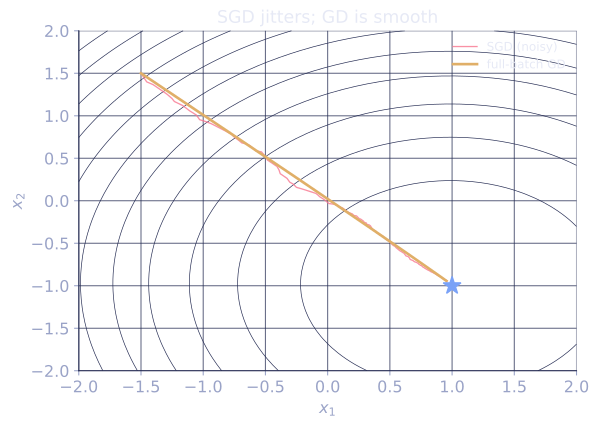
Machine-learning objectives are averages over millions of examples, and computing the full gradient every step is prohibitive. Stochastic gradient descent replaces it with the gradient of a small random batch: a noisy but unbiased and cheap estimate. The noise changes the convergence story, and managing it through the step-size schedule is the central practical skill.

The finite-sum objective

Training minimizes an average loss over $n$ examples,

where $f_i$ is the loss on example $i$ and $x$ are the parameters. The full gradient $\nabla f(x) = \frac{1}{n}\sum_i \nabla f_i(x)$ costs a pass over all $n$ examples.

The stochastic update

SGD samples an index $i_t$ (or a small minibatch) uniformly at random and steps along that single gradient:

The key property is unbiasedness: averaging over the random draw,

The stochastic gradient points in the right direction on average, but any single step is corrupted by variance $\sigma^2 = \mathbb{E}\lVert \nabla f_{i_t}(x) - \nabla f(x)\rVert^2$.

The noise floor with a constant step size

The variance changes convergence fundamentally. For $\mu$-strongly convex, $L$-smooth $f$ with a constant step size $\eta$, the expected suboptimality satisfies a recursion of the form

The first term contracts as in deterministic GD; the second injects noise every step. At the fixed point, contraction balances injection and the iterates hover at a noise floor:

Constant-step SGD converges fast to a neighborhood of the optimum, then bounces around it. The floor height is proportional to $\eta$: a smaller step gives a lower floor but slower approach.

Decaying step sizes

To reach the exact optimum, the step size must shrink so the noise term vanishes. The Robbins-Monro conditions are

A schedule like $\eta_t = \eta_0 / t$ satisfies both and gives $\mathbb{E}[\Delta_t] = O(1/t)$. In practice, step decay or cosine schedules implement the same idea: large steps early to move fast, small steps late to settle.

Why minibatches

A minibatch of size $B$ averages $B$ independent gradient estimates, cutting the variance to $\sigma^2 / B$. This lowers the noise floor and lets a larger step size be used, while exploiting vectorized hardware. The minibatch size trades gradient quality against per-step cost.

Check it on arrays

import numpy as np

rng = np.random.default_rng(0)

# Least squares as a finite sum: f_i(x) = 0.5 (a_i^T x - b_i)^2
n, d = 2000, 10
A = rng.normal(size=(n, d))
x_true = rng.normal(size=d)
b = A @ x_true + 0.1 * rng.normal(size=n)
x_star = np.linalg.lstsq(A, b, rcond=None)[0]

def full_loss(x):
    return 0.5 * np.mean((A @ x - b)**2)

def sgd(eta, batch=1, steps=20_000, decay=False):
    x = np.zeros(d)
    for t in range(steps):
        idx = rng.integers(0, n, size=batch)
        g = A[idx].T @ (A[idx] @ x - b[idx]) / batch
        lr = eta / (1 + 0.001 * t) if decay else eta
        x = x - lr * g
    return full_loss(x) - full_loss(x_star)

# Constant step: lower eta -> lower noise floor
print("const eta=0.05, B=1 :", round(sgd(0.05), 6))
print("const eta=0.01, B=1 :", round(sgd(0.01), 6))
# Bigger batch lowers the floor at the same step size
print("const eta=0.05, B=32:", round(sgd(0.05, batch=32), 6))
# Decaying step reaches lower suboptimality
print("decaying eta0=0.05  :", round(sgd(0.05, decay=True), 6))

A smaller constant step and a larger batch both lower the noise floor, and the decaying schedule drives suboptimality further down.

Exercises

Exercise 1. A constant-step SGD run with step $\eta$ settles at a noise floor of height $\frac{\eta L \sigma^2}{2\mu}$. If halving the step is observed to halve the floor, explain why, and predict the floor after dividing the step by $10$ relative to the original.

Exercise 2. Show that the minibatch gradient is unbiased and that a batch of size $B$ drawn with replacement has variance $\sigma^2 / B$. Let $g_B = \frac{1}{B}\sum_{j=1}^B \nabla f_{i_j}(x)$ with the $i_j$ independent and uniform.

Exercise 3 (code). Estimate the noise floor empirically. Run constant-step SGD on a least-squares finite sum, and verify that halving the step size roughly halves the measured suboptimality floor, matching the linear $\eta$ dependence of Exercise 1.

import numpy as np

rng = np.random.default_rng(0)
n, d = 2000, 10
A = rng.normal(size=(n, d))
x_true = rng.normal(size=d)
b = A @ x_true + 0.1 * rng.normal(size=n)
x_star = np.linalg.lstsq(A, b, rcond=None)[0]

def full_loss(x):
    return 0.5 * np.mean((A @ x - b)**2)

def floor(eta, steps=40_000, tail=5_000):
    # average suboptimality over the last `tail` steps = noise-floor estimate
    x = np.zeros(d)
    acc = 0.0
    for t in range(steps):
        i = rng.integers(0, n)
        g = A[i] * (A[i] @ x - b[i])
        x = x - eta * g
        if t >= steps - tail:
            acc += full_loss(x) - full_loss(x_star)
    return acc / tail

f1 = floor(0.02)
f2 = floor(0.01)                                 # half the step
ratio = f2 / f1
print("floor(eta=0.02):", round(f1, 6))
print("floor(eta=0.01):", round(f2, 6))
print("ratio:", round(ratio, 3))

assert 0.35 < ratio < 0.75                       # near 0.5, the linear prediction

The next lesson speeds up the deterministic part with momentum.

References

- [1]Goodfellow, I., Bengio, Y., & Courville, A. (2016). Deep Learning, ch. 8. MIT Press. Minibatch stochastic gradient estimates and their unbiasedness.↩
- [2]Robbins, H., & Monro, S. (1951). "A stochastic approximation method". Annals of Mathematical Statistics, 22, 400-407. The step-size conditions for convergence (doi:10.1214/aoms/1177729586).↩