Smoothness, strong convexity, and convergence rates

The descent lemma says gradient descent makes progress; it does not say how fast. The speed depends on two curvature bounds: an upper bound (smoothness) that caps how large a step is safe, and a lower bound (strong convexity) that guarantees the function is not too flat. Their ratio, the condition number, sets the rate.

The two curvature bounds

$f$ is $L$-smooth if $\nabla^2 f \preceq L I$ (curvature at most $L$), giving the quadratic upper bound from the previous lesson. $f$ is $\mu$-strongly convex if $\nabla^2 f \succeq \mu I$ for some $\mu > 0$, equivalently

The function is sandwiched between two quadratics: $\mu I \preceq \nabla^2 f \preceq L I$. Strong convexity forces a unique minimizer and a paraboloid-like bowl no flatter than curvature $\mu$.

The Polyak-Lojasiewicz inequality

Strong convexity implies a bound relating the suboptimality to the gradient norm. Minimizing both sides of the strong-convexity inequality over $y$ (the right side is a quadratic in $y$, minimized at $y = x - \frac{1}{\mu}\nabla f(x)$) gives

A small objective gap forces a small gradient and vice versa: there are no flat near-optimal plateaus to stall on.

Linear convergence for strongly convex, smooth $f$

Combine the descent lemma (with $\eta = 1/L$) and the PL inequality. Let $\Delta_t = f(x_t) - f(x^\star)$. The descent lemma gives $\Delta_{t+1} \le \Delta_t - \frac{1}{2L}\lVert\nabla f(x_t)\rVert^2$, and PL bounds the gradient term below by $2\mu\Delta_t$:

Iterating,

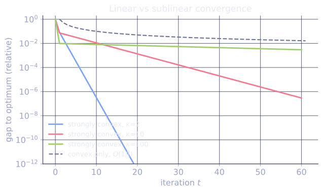
This is linear convergence: the gap shrinks by a constant factor each step, so reaching accuracy $\varepsilon$ takes $O\!\big(\frac{L}{\mu}\log\frac{1}{\varepsilon}\big)$ iterations.

The condition number

The ratio

is the condition number of the problem. It controls everything: the rate factor is $1 - 1/\kappa$, so a well-conditioned problem ($\kappa$ near 1) converges in few steps, while an ill-conditioned one ($\kappa$ large) crawls because the safe step size $1/L$ is tiny relative to the gentle curvature $\mu$ along the flat directions. For a quadratic, $\kappa$ is the ratio of largest to smallest Hessian eigenvalue, the same condition number from the SVD.

To feel what $\kappa$ buys, count the steps to shrink the gap to $\varepsilon = 10^{-6}$, which is $\log\varepsilon / \log(1 - 1/\kappa)$ steps:

• $\kappa = 2$ (nearly round bowl): factor $1 - 1/2 = 0.5$, about 20 steps. The gap halves every iteration.
• $\kappa = 10$: factor $0.9$, about 131 steps.
• $\kappa = 100$: factor $0.99$, about 1375 steps.
• $\kappa = 1000$ (a ravine 1000 times steeper across than along): factor $0.999$, about 13800 steps.

The cost grows roughly in proportion to $\kappa$: each tenfold worsening of the conditioning multiplies the step count by about ten. The three runs in the code below ($\kappa = 2, 10, 100$) trace the first three rows.

Sublinear rate without strong convexity

If $f$ is convex and $L$-smooth but not strongly convex ($\mu = 0$), the rate drops to

an $O(1/t)$ sublinear rate. Reaching $\varepsilon$ now takes $O(1/\varepsilon)$ steps, far more than the $\log(1/\varepsilon)$ of the strongly convex case. The lower curvature bound is what buys the exponential speedup.

Check it on arrays

import numpy as np

# Quadratic with controllable conditioning: f(x) = 0.5 x^T A x, A = diag(mu, L)
def run(mu, L, steps=200):
    A = np.diag([mu, L])
    grad = lambda x: A @ x
    eta = 1.0 / L
    x = np.array([1.0, 1.0])
    gaps = []
    for _ in range(steps):
        gaps.append(0.5 * x @ A @ x)             # f(x*) = 0
        x = x - eta * grad(x)
    return np.array(gaps)

for mu, L in [(1.0, 2.0), (1.0, 10.0), (1.0, 100.0)]:
    gaps = run(mu, L)
    kappa = L / mu
    # empirical contraction factor vs predicted (1 - 1/kappa)
    ratio = (gaps[100] / gaps[50]) ** (1 / 50)
    print(f"kappa={kappa:>5.0f}: empirical factor {ratio:.4f}, "
          f"predicted <= {1 - 1/kappa:.4f}")

The per-step contraction factor stays at or below the predicted $1 - 1/\kappa$, and worsens as the condition number grows.

Exercises

Exercise 1. A problem is $L$-smooth with $L = 20$ and $\mu$-strongly convex with $\mu = 2$. Compute the condition number $\kappa$, the linear-rate contraction factor $1 - \mu/L$, and the number of steps the bound predicts to shrink the gap to $\varepsilon = 10^{-6}$ of its starting value.

Exercise 2. Derive the PL inequality $\lVert \nabla f(x)\rVert^2 \ge 2\mu\,(f(x) - f(x^\star))$ from the strong-convexity inequality. Show each step.

Exercise 3 (code). For the diagonal quadratic $f(x) = \tfrac12 x^\top A x$ with $A = \mathrm{diag}(\mu, L)$, $\mu = 1$, $L = 50$, run gradient descent with step $\eta = 1/L$ from $x_0 = (1, 1)$. Confirm the gap shrinks by no more than the predicted factor $1 - 1/\kappa$ per step, and that the bound $\Delta_t \le (1 - 1/\kappa)^t \Delta_0$ holds at $t = 100$.

import numpy as np

mu, L = 1.0, 50.0
kappa = L / mu
A = np.diag([mu, L])
eta = 1.0 / L

x = np.array([1.0, 1.0])
f = lambda z: 0.5 * z @ A @ z          # f(x*) = 0, so gap = f(x)
gaps = [f(x)]
for _ in range(100):
    x = x - eta * (A @ x)
    gaps.append(f(x))
gaps = np.array(gaps)

factors = gaps[1:] / gaps[:-1]
assert np.all(factors <= (1 - 1/kappa) + 1e-9)          # per-step contraction
assert gaps[100] <= (1 - 1/kappa)**100 * gaps[0] + 1e-12  # iterated bound
print("worst per-step factor:", round(factors.max(), 4),
      " predicted bound:", round(1 - 1/kappa, 4))

The next lesson replaces the full gradient with a noisy estimate, the stochastic setting of real training.

References

- [1]Nesterov, Y. (2018). Lectures on Convex Optimization (2nd ed.), §2.1. Springer. Smoothness, strong convexity, and the linear rate for gradient descent.↩
- [2]Nocedal, J., & Wright, S. J. (2006). Numerical Optimization (2nd ed.), §3.3. Springer. Convergence rates and the role of the condition number (doi:10.1007/978-0-387-40065-5).↩