Quasi-Newton methods (BFGS, L-BFGS)

Newton's method is fast but pays $O(n^3)$ per step to invert the Hessian, and often the Hessian is unavailable anyway. Quasi-Newton methods build an approximation to the inverse Hessian from nothing but the gradients already computed, recovering most of Newton's speed at gradient-descent cost. BFGS and its limited-memory form L-BFGS are the workhorses of classical smooth optimization.

The secant condition

The idea is to infer curvature from how the gradient changes. Over one step define

For a quadratic with Hessian $H$, the gradient change is exactly $y_t = H s_t$. A quasi-Newton method requires its Hessian approximation $B_{t+1}$ to reproduce this observed relationship, the secant condition:

This is the multidimensional analogue of estimating a second derivative from two first derivatives. One equation underdetermines the $n \times n$ matrix, so the method adds a requirement that $B_{t+1}$ stay close to $B_t$.

The BFGS update

BFGS updates the inverse Hessian approximation $H_t \approx [\nabla^2 f]^{-1}$ directly, so each step needs only a matrix-vector product, not a solve. With $\rho_t = 1/(y_t^\top s_t)$:

This is a rank-two correction to $H_t$ chosen to satisfy the secant condition while keeping $H_{t+1}$ symmetric. As long as the curvature condition $y_t^\top s_t > 0$ holds (guaranteed by a proper line search), the update preserves positive definiteness, so the search direction $-H_t \nabla f(x_t)$ is always a descent direction. The step is

with $\alpha_t$ from a line search. BFGS converges superlinearly: faster than any linear rate, approaching Newton, without ever forming a Hessian.

L-BFGS: limited memory

Storing the dense $n \times n$ matrix $H_t$ is $O(n^2)$, still too much for large $n$. L-BFGS never forms $H_t$. It keeps only the last $m$ pairs $(s_k, y_k)$ (typically $m = 5$ to $20$) and computes the product $H_t \nabla f(x_t)$ on the fly with the two-loop recursion: one backward pass over the stored pairs applying the $(I - \rho s y^\top)$ factors, a scaling by an estimate of the Hessian, then one forward pass. Cost and memory drop to $O(mn)$, linear in the dimension. L-BFGS is the default for medium-scale smooth problems and large-batch training where the gradients are clean enough to trust[2].

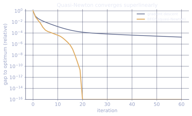
Check it on arrays

import numpy as np

# Minimize f(x) = 0.5 x^T A x - b^T x with BFGS (inverse-Hessian form).
rng = np.random.default_rng(0)
n = 20
Q = np.linalg.qr(rng.normal(size=(n, n)))[0]
A = Q @ np.diag(np.linspace(1.0, 50.0, n)) @ Q.T   # SPD, condition number 50
b = rng.normal(size=n)
x_star = np.linalg.solve(A, b)

f = lambda x: 0.5 * x @ A @ x - b @ x
grad = lambda x: A @ x - b

def line_search(x, p):                              # backtracking (Armijo)
    a, g = 1.0, grad(x)
    while f(x + a * p) > f(x) + 1e-4 * a * (g @ p):
        a *= 0.5
    return a

x = np.zeros(n)
H = np.eye(n)                                       # initial inverse-Hessian guess
g = grad(x)
for t in range(40):
    p = -H @ g
    alpha = line_search(x, p)
    s = alpha * p
    x_new = x + s
    g_new = grad(x_new)
    y = g_new - g
    rho = 1.0 / (y @ s)
    if y @ s > 1e-12:                               # curvature condition
        I = np.eye(n)
        H = (I - rho * np.outer(s, y)) @ H @ (I - rho * np.outer(y, s)) + rho * np.outer(s, s)
    x, g = x_new, g_new

print("BFGS error:", f"{np.linalg.norm(x - x_star):.2e}")
print("gradient norm:", f"{np.linalg.norm(g):.2e}")

BFGS reaches the minimizer of an ill-conditioned ($\kappa = 50$) quadratic in a few dozen steps using only gradients, with the inverse-Hessian estimate built from the secant pairs.

Exercises

Exercise 1. On a quadratic $f(x) = \tfrac12 x^\top H x - b^\top x$, take one step $s_t = x_{t+1} - x_t$ and form $y_t = \nabla f(x_{t+1}) - \nabla f(x_t)$. Show by hand that the secant condition $H s_t = y_t$ holds exactly, so the true Hessian satisfies the constraint BFGS imposes.

Exercise 2. The curvature condition $y_t^\top s_t > 0$ guarantees BFGS keeps its inverse-Hessian estimate positive definite. Show that for a strictly convex quadratic with Hessian $H \succ 0$, the curvature condition holds for any nonzero step $s_t$.

Exercise 3 (code). Implement the L-BFGS two-loop recursion that computes the product $H_t \nabla f$ from the last $m$ stored pairs $(s_k, y_k)$, without ever forming a matrix. Verify it against the dense BFGS inverse-Hessian on the same pairs by checking the two search directions agree.

import numpy as np

rng = np.random.default_rng(0)
n, m = 12, 5

# Build m secant pairs from a fixed SPD Hessian so curvature condition holds.
M = rng.normal(size=(n, n)); H_true = M @ M.T + n * np.eye(n)
S = rng.normal(size=(m, n))
Y = S @ H_true                                  # y_k = H s_k (rows)

# Dense BFGS inverse-Hessian built from the same pairs (gamma * I start).
gamma = (S[-1] @ Y[-1]) / (Y[-1] @ Y[-1])
Hdense = gamma * np.eye(n)
for k in range(m):
    s, y = S[k], Y[k]
    rho = 1.0 / (y @ s)
    I = np.eye(n)
    Hdense = (I - rho * np.outer(s, y)) @ Hdense @ (I - rho * np.outer(y, s)) + rho * np.outer(s, s)

g = rng.normal(size=n)
dense_dir = Hdense @ g

# Two-loop recursion: same H0 = gamma * I, same pairs, applied implicitly.
def two_loop(g, S, Y, gamma):
    q = g.copy()
    alpha = np.zeros(m)
    rho = np.array([1.0 / (Y[k] @ S[k]) for k in range(m)])
    for k in reversed(range(m)):                # backward pass
        alpha[k] = rho[k] * (S[k] @ q)
        q = q - alpha[k] * Y[k]
    r = gamma * q                               # H0 * q
    for k in range(m):                          # forward pass
        beta = rho[k] * (Y[k] @ r)
        r = r + (alpha[k] - beta) * S[k]
    return r

loop_dir = two_loop(g, S, Y, gamma)

assert np.allclose(loop_dir, dense_dir, atol=1e-8)
print("max abs difference:", float(np.max(np.abs(loop_dir - dense_dir))))

The next lesson handles objectives that are not smooth, with proximal methods.

References

- [1]Nocedal, J., & Wright, S. J. (2006). Numerical Optimization (2nd ed.), §6.1. Springer. The secant condition and the BFGS inverse-Hessian update (doi:10.1007/978-0-387-40065-5).↩
- [2]Nocedal, J., & Wright, S. J. (2006). Numerical Optimization (2nd ed.), §7.2. Springer. Limited-memory L-BFGS and the two-loop recursion.↩