AdaGrad, RMSProp, and Adam

A single global step size is a poor fit when coordinates have wildly different curvatures or gradient scales, as they do across the layers of a deep network. Adaptive methods give each coordinate its own effective step size, derived from the history of its gradients. Adam, the default optimizer for most deep learning, combines this idea with momentum.

AdaGrad: accumulate squared gradients

AdaGrad divides each coordinate's step by the square root of its accumulated squared gradient. With $g_t = \nabla f(x_t)$ and elementwise operations:

Coordinates with large or frequent gradients get a shrinking step; rarely updated coordinates keep a large one. The $\epsilon$ (a tiny constant like $10^{-8}$) prevents division by zero. The flaw: $G_t$ only grows, so the effective step decays monotonically to zero and learning stalls on long runs.

RMSProp: forget the distant past

RMSProp fixes the monotone decay by replacing the running sum with an exponentially weighted moving average of squared gradients, decaying old information with rate $\rho$ (typically 0.9):

Because $S_t$ tracks a window rather than all history, the effective step size adapts to the recent gradient scale and does not collapse. This makes RMSProp suitable for nonstationary objectives where the right scale changes during training.

Adam: momentum plus RMSProp

Adam maintains two moving averages: a first moment $m_t$ (momentum, the mean gradient) and a second moment $v_t$ (the RMSProp scale), with decay rates $\beta_1$ (0.9) and $\beta_2$ (0.999):

Initialized at zero, both averages are biased toward zero early on. Adam corrects this with bias correction, dividing by $1 - \beta^t$:

Why the correction. With $m_0 = 0$, the average $m_t = (1-\beta_1)\sum_{k=1}^t \beta_1^{t-k}g_k$ has expectation about $(1 - \beta_1^t)\,\mathbb{E}[g]$, underestimating by the factor $1 - \beta_1^t$. Dividing by it restores an unbiased estimate, important in the first few steps when $\beta_1^t$ is not yet negligible. The final update is

AdamW decouples weight decay from the adaptive step, applying the L2 penalty directly to the weights ($x_{t+1} \mathrel{-}= \eta\lambda x_t$) rather than folding it into the gradient, which interacts badly with the $\sqrt{\hat v_t}$ rescaling. AdamW is the standard for training transformers.

Check it on arrays

import numpy as np

rng = np.random.default_rng(0)

# Badly scaled quadratic: coordinate curvatures span 3 orders of magnitude.
scales = np.array([1.0, 10.0, 100.0, 1000.0])
f = lambda x: 0.5 * np.sum(scales * x**2)
grad = lambda x: scales * x

def adam(steps=500, eta=0.1, b1=0.9, b2=0.999, eps=1e-8):
    x = np.ones(4); m = np.zeros(4); v = np.zeros(4)
    for t in range(1, steps + 1):
        g = grad(x)
        m = b1 * m + (1 - b1) * g
        v = b2 * v + (1 - b2) * g**2
        mhat = m / (1 - b1**t)
        vhat = v / (1 - b2**t)
        x = x - eta * mhat / (np.sqrt(vhat) + eps)
    return f(x)

def plain_gd(steps=500, eta=1.0 / 1000):           # eta limited by largest curvature
    x = np.ones(4)
    for _ in range(steps):
        x = x - eta * grad(x)
    return f(x)

print("Adam final f:    ", f"{adam():.3e}")
print("plain GD final f:", f"{plain_gd():.3e}")   # crawls on the flat coordinate

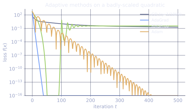
Adam drives every coordinate down despite the 1000x curvature spread, while plain gradient descent, capped by the steepest coordinate, barely moves the flattest one.

Exercises

Exercise 1. Adam runs with $\beta_1 = 0.9$ and $\beta_2 = 0.999$. Compute the bias-correction factors $1 - \beta_1^t$ and $1 - \beta_2^t$ at $t = 1$ and at $t = 10$, and explain why the second-moment correction matters for longer than the first.

Exercise 2. Consider one coordinate where the gradient is the constant $g$ at every step. Show that AdaGrad's effective step size $\eta / (\sqrt{G_t} + \epsilon)$ decays like $1/\sqrt{t}$, while RMSProp's reaches a finite steady value. Ignore $\epsilon$.

Exercise 3 (code). Implement RMSProp and confirm Step 2 of Exercise 2 numerically: with a constant gradient $g = 2$ and $\rho = 0.9$, the running average $S_t$ converges to $g^2 = 4$ and the effective step converges to $\eta / |g|$.

import numpy as np

g = 2.0
rho = 0.9
eta = 0.1
eps = 1e-8

S = 0.0
for _ in range(500):
    S = rho * S + (1 - rho) * g**2     # constant gradient each step

eff_step = eta / (np.sqrt(S) + eps)

assert np.isclose(S, g**2, atol=1e-6)             # S_inf = g^2 = 4
assert np.isclose(eff_step, eta / abs(g), atol=1e-6)
print("S_inf:", round(S, 6), " effective step:", round(eff_step, 6))

The next lesson turns from unconstrained methods to optimization under constraints.

References

- [1]Duchi, J., Hazan, E., & Singer, Y. (2011). "Adaptive subgradient methods for online learning and stochastic optimization (AdaGrad)". JMLR, 12, 2121-2159. The per-coordinate accumulated-gradient step size.↩
- [2]Kingma, D. P., & Ba, J. (2015). "Adam: A method for stochastic optimization". ICLR. The first/second-moment update with bias correction (arXiv:1412.6980).↩
- [3]Goodfellow, I., Bengio, Y., & Courville, A. (2016). Deep Learning, ch. 8. MIT Press. A comparative treatment of RMSProp, Adam, and related adaptive optimizers.↩