Diagonalization & the spectral theorem

Diagonalization turns $n$ coupled equations into $n$ independent ones, and symmetric matrices are the class where diagonalization is always possible with an orthonormal basis. This is the spectral theorem, the cornerstone of PCA, covariance analysis, and quadratic-form optimization.

Diagonalization

A matrix $A \in \mathbb{R}^{n \times n}$ is diagonalizable if there exist an invertible matrix $P$ and a diagonal matrix $\Lambda$ such that

The columns of $P$ are eigenvectors of $A$ (column $j$ of $AP = P\Lambda$ says $Ap_j = \lambda_j p_j$), and the diagonal entries of $\Lambda$ are the corresponding eigenvalues.

A matrix is diagonalizable if and only if it has $n$ linearly independent eigenvectors. Eigenvectors from distinct eigenvalues are automatically independent (proof below), so a matrix with $n$ distinct eigenvalues is diagonalizable.

Independence of eigenvectors for distinct eigenvalues. Suppose $A v_i = \lambda_i v_i$ for $i = 1, \dots, k$ with $\lambda_i$ all different, and suppose $\sum c_i v_i = 0$. Apply $A - \lambda_1 I$ to both sides: $\sum_{i=2}^k c_i(\lambda_i - \lambda_1) v_i = 0$. Repeat with $A - \lambda_2 I$, and so on, until you isolate each $c_i$ multiplying a nonzero vector; each must be zero. By induction, $c_i = 0$ for all $i$.

The spectral theorem for real symmetric matrices

Theorem. If $A \in \mathbb{R}^{n \times n}$ is symmetric ($A = A^\top$), then[1, 2]:

1. All eigenvalues of $A$ are real.
2. Eigenvectors for distinct eigenvalues are orthogonal.
3. There exists an orthonormal basis of $\mathbb{R}^n$ consisting of eigenvectors of $A$.

Proof of (1): eigenvalues are real. Let $\lambda$ be an eigenvalue (possibly complex) with eigenvector $v \in \mathbb{C}^n$ (possibly complex). Using the conjugate transpose $\bar{v}^\top$:

Since $v \neq 0$, $\bar{v}^\top v = \lVert v\rVert^2 > 0$, so $\lambda = \bar\lambda$, meaning $\lambda$ is real.

Proof of (2): eigenvectors for distinct eigenvalues are orthogonal. Let $Av_1 = \lambda_1 v_1$ and $Av_2 = \lambda_2 v_2$ with $\lambda_1 \neq \lambda_2$. Then:

So $(\lambda_1 - \lambda_2)\langle v_1, v_2\rangle = 0$; since $\lambda_1 \neq \lambda_2$, the inner product is zero.

Proof of (3) (sketch): induct on $n$. For $n=1$ it is trivial. For $n > 1$: pick any real eigenvalue $\lambda_1$ (guaranteed by (1)) with eigenvector $q_1$ (normalized). The subspace $W = q_1^\perp$ is invariant under $A$: if $w \perp q_1$ then $\langle Aw, q_1\rangle = \langle w, Aq_1\rangle = \lambda_1\langle w, q_1\rangle = 0$. Restrict $A$ to $W$ (an $(n-1)$-dimensional symmetric operator), apply the induction hypothesis, and concatenate. $\qquad\blacksquare$

The spectral decomposition

Collecting the orthonormal eigenbasis into columns of $Q$:

where $Q^\top Q = I$ and $\Lambda = \operatorname{diag}(\lambda_1, \dots, \lambda_n)$.

Expanding:

Each term $q_i q_i^\top$ is the projection matrix onto the $i$-th eigenvector direction. The matrix $A$ is a weighted sum of rank-1 projections, with weights given by the eigenvalues.

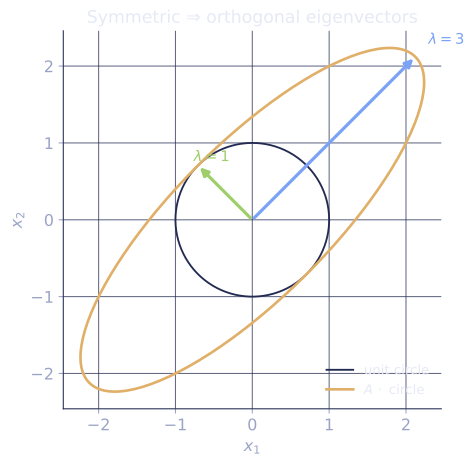
Check it on arrays

import numpy as np

# A real symmetric matrix
A = np.array([[4.0, 2.0, 0.0],
              [2.0, 3.0, 1.0],
              [0.0, 1.0, 2.0]])

eigenvalues, Q = np.linalg.eigh(A)   # eigh exploits symmetry: real output, sorted
print("eigenvalues:", np.round(eigenvalues, 6))

# Verify Q is orthogonal
print("Q^T Q:\n", np.round(Q.T @ Q, 10))   # identity

# Reconstruct: A = Q Lam Q^T
A_reconstructed = Q @ np.diag(eigenvalues) @ Q.T
print("reconstruction error:", np.max(np.abs(A - A_reconstructed)))   # ~1e-15

# Spectral decomposition: sum of rank-1 projections
A_spectral = sum(lam * np.outer(Q[:, i], Q[:, i])
                 for i, lam in enumerate(eigenvalues))
print("spectral sum error:", np.max(np.abs(A - A_spectral)))   # ~1e-15

The reconstruction from the spectral decomposition recovers $A$ to machine precision.

Exercises

Exercise 1. Diagonalize $A = \begin{bmatrix} 2 & 1 \\ 1 & 2 \end{bmatrix}$ by hand: find its eigenvalues and an orthonormal eigenbasis, and write $A = Q\Lambda Q^\top$.

Exercise 2. Using the spectral decomposition $A = \sum_i \lambda_i q_i q_i^\top$, prove that $\operatorname{tr}(A) = \sum_i \lambda_i$ for a symmetric $A$.

Exercise 3 (code). For a random symmetric $4 \times 4$ matrix, verify with np.linalg.eigh that (i) the eigenvalues are real, (ii) the eigenvector matrix $Q$ is orthogonal, and (iii) eigenvectors for distinct eigenvalues are orthogonal.

import numpy as np

rng = np.random.default_rng(0)
M = rng.normal(size=(4, 4))
A = 0.5 * (M + M.T)                      # symmetric

w, Q = np.linalg.eigh(A)

# (i) eigenvalues are real: eigh returns real arrays for symmetric input.
assert np.isrealobj(w)

# (ii) Q is orthogonal: Q^T Q = I.
assert np.allclose(Q.T @ Q, np.eye(4), atol=1e-12)

# (iii) distinct eigenvalues -> orthogonal eigenvectors (off-diagonals ~ 0).
gram = Q.T @ Q
assert np.allclose(gram - np.diag(np.diag(gram)), 0, atol=1e-12)
print("eigenvalues:", np.round(w, 6))

The eigenvalue signs in that decomposition determine whether the associated quadratic form is positive definite, the subject of the next lesson.

References

- [1]Axler, S. (2015). Linear Algebra Done Right (3rd ed.), ch. 7. Springer. The spectral theorem for self-adjoint operators (doi:10.1007/978-3-319-11080-6).↩
- [2]Horn, R. A., & Johnson, C. R. (2012). Matrix Analysis (2nd ed.). Cambridge University Press. Diagonalization and the spectral decomposition of symmetric matrices.↩