Optimization problems, minima, and gradients

Training a model is minimizing a loss. Before any algorithm, the question is what a solution even is: where are the minima of a function, how do you recognize one, and what distinguishes a true minimum from a saddle? The gradient and the Hessian answer this locally, and they are the only information first- and second-order methods ever use.

The problem

An unconstrained optimization problem is

where $f: \mathbb{R}^n \to \mathbb{R}$ is the objective. A point $x^\star$ is a global minimum if $f(x^\star) \le f(x)$ for all $x$, and a local minimum if the inequality holds only in a neighborhood. Optimization algorithms find local minima; extra structure (convexity, a later lesson) is what promotes them to global.

First-order condition

At a smooth interior minimum the gradient vanishes. The gradient

points in the direction of steepest ascent, and its negative is steepest descent.

Theorem (necessary condition). If $x^\star$ is a local minimum and $f$ is differentiable there, then $\nabla f(x^\star) = 0$.

Proof. Along any direction $d$, the function $g(t) = f(x^\star + td)$ has a local minimum at $t = 0$, so $g'(0) = \nabla f(x^\star)^\top d = 0$. Since this holds for every $d$, the gradient must be the zero vector. $\qquad\blacksquare$[1]

A point with $\nabla f = 0$ is a stationary point. It can be a minimum, a maximum, or a saddle; the first-order condition alone cannot tell them apart.

Second-order condition

The Hessian $\nabla^2 f(x)$ is the symmetric matrix of second partials, $[\nabla^2 f]_{ij} = \partial^2 f / \partial x_i \partial x_j$. It is the local curvature. Expanding $f$ to second order around a stationary point $x^\star$:

since the gradient term drops. The sign of the quadratic form $d^\top \nabla^2 f\, d$ decides the type, using the definiteness language from quadratic forms:

• $\nabla^2 f(x^\star) \succ 0$ (positive definite): every direction curves up, a strict local minimum.
• $\nabla^2 f(x^\star) \prec 0$ (negative definite): a local maximum.
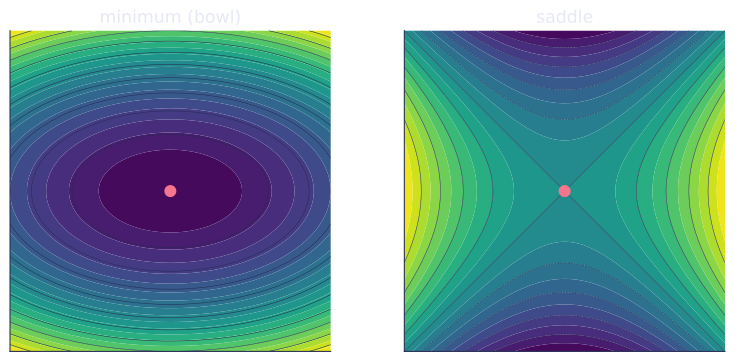
• Indefinite (mixed eigenvalue signs): a saddle point, a minimum along some directions and a maximum along others.

Saddles, not bad local minima, are the dominant stationary points of high-dimensional loss surfaces, which shapes how neural-network optimizers behave[2].

Directional derivatives and descent directions

A direction $d$ is a descent direction at $x$ if $\nabla f(x)^\top d < 0$: moving slightly along $d$ decreases $f$, because the directional derivative is negative. The steepest descent direction is $d = -\nabla f(x)$, the choice the next lessons build on.

Check it on arrays

import numpy as np

# f(x,y) = x^2 + 3y^2 (bowl): minimum at origin, Hessian = diag(2,6) > 0
def f(v): return v[0]**2 + 3*v[1]**2
def grad(v): return np.array([2*v[0], 6*v[1]])
def hess(v): return np.array([[2.0, 0.0], [0.0, 6.0]])

x0 = np.array([0.0, 0.0])
print("grad at origin:", grad(x0), " (stationary)")
eig = np.linalg.eigvalsh(hess(x0))
print("Hessian eigenvalues:", eig, "-> all > 0 -> local min")

# A saddle: g(x,y) = x^2 - y^2, Hessian = diag(2,-2) indefinite
def hess_saddle(v): return np.array([[2.0, 0.0], [0.0, -2.0]])
print("saddle Hessian eigenvalues:", np.linalg.eigvalsh(hess_saddle(x0)),
      "-> mixed signs -> saddle")

# Descent direction check: -grad should have negative directional derivative
x = np.array([1.0, 1.0])
d = -grad(x)
print("grad . d =", grad(x) @ d, "< 0 -> descent direction")

# Finite-difference gradient check
eps = 1e-6
fd = np.array([(f(x + eps*np.eye(2)[i]) - f(x - eps*np.eye(2)[i]))/(2*eps) for i in range(2)])
print("analytic grad:", grad(x), " finite-diff:", np.round(fd, 6))

The bowl's Hessian is positive definite (a minimum), the saddle's is indefinite, the negative gradient is a descent direction, and finite differences confirm the analytic gradient.

Exercises

Exercise 1. For $f(x, y) = x^2 + 3y^2$, find every stationary point by hand, then classify it using the Hessian. Confirm it is a strict local minimum.

Exercise 2. The first-order condition $\nabla f(x^\star) = 0$ is necessary but not sufficient. Show that $f(x, y) = x^2 - y^2$ has a stationary point at the origin that is neither a minimum nor a maximum, and identify the directions of increase and decrease.

Exercise 3 (code). Pick a random symmetric $5 \times 5$ matrix as a Hessian and the quadratic $f(d) = \tfrac12 d^\top H d$. Verify numerically that $d = -\nabla f(x)$ is a descent direction at a nonzero $x$ whenever the directional derivative $\nabla f(x)^\top d$ is negative, and that this holds at every nonzero point.

import numpy as np

rng = np.random.default_rng(0)
M = rng.normal(size=(5, 5))
H = M + M.T                                  # symmetric Hessian (any signature)

# f(x) = 0.5 x^T H x, grad = H x (H symmetric)
grad = lambda x: H @ x

# At many random nonzero points, -grad is a descent direction unless grad == 0.
ratios = []
for _ in range(1000):
    x = rng.normal(size=5)
    g = grad(x)
    d = -g
    dd = g @ d                               # directional derivative along -grad
    ratios.append(dd / (g @ g))              # equals -1 whenever grad != 0
    assert dd <= 0                           # never an ascent direction

# -grad gives directional derivative -||grad||^2 <= 0, strictly < 0 when grad != 0.
ratios = np.array(ratios)
assert np.allclose(ratios, -1.0)
print("directional derivative ratio (all):", round(ratios.max(), 6))

The next lesson defines the geometric property, convexity, that makes a stationary point a global minimum.