Proximal gradient methods

Define the proximal operator and use proximal gradient descent for nonsmooth objectives like the L1 penalty.

⏱ 32 minPrerequisites:Gradient descent Convex functions and their tests

Gradient descent needs a gradient, but the most useful regularizer, the L1 penalty that produces sparsity, is not differentiable at zero. Proximal methods split the objective into a smooth part and a simple nonsmooth part, taking a gradient step on the first and a proximal step on the second. For the L1 penalty the proximal step is soft-thresholding, and the result is the LASSO solver ISTA.

The composite problem

Many learning objectives have the form

\min_x\; \underbrace{f(x)}_{\text{smooth}} + \underbrace{g(x)}_{\text{nonsmooth, simple}},

where $f$ is convex and $L$ -smooth (a data-fit loss) and $g$ is convex but possibly nondifferentiable (a regularizer like $\lambda\lVert x\rVert_1$ ). Plain gradient descent fails on $g$ ; the proximal operator handles it exactly.

The proximal operator

The proximal operator of a function $g$ with step $\eta$ is

\operatorname{prox}_{\eta g}(v) = \arg\min_x\left(g(x) + \frac{1}{2\eta}\lVert x - v\rVert^2\right).

[1]

It returns the point that balances minimizing $g$ against staying near $v$ . It generalizes projection: if $g$ is the indicator of a convex set (zero inside, $+\infty$ outside), the prox is exactly Euclidean projection onto that set.

Proximal gradient descent

Proximal gradient descent alternates a gradient step on $f$ with a prox step on $g$ :

x_{t+1} = \operatorname{prox}_{\eta g}\!\big(x_t - \eta\,\nabla f(x_t)\big).

The motivation mirrors the gradient-descent derivation: model $f$ by its linearization plus a proximity penalty, keep $g$ exact, and minimize. The minimizer of $f(x_t) + \nabla f(x_t)^\top(x - x_t) + \frac{1}{2\eta}\lVert x - x_t\rVert^2 + g(x)$ is precisely the prox of $g$ applied to the gradient step. With $\eta \le 1/L$ it converges at the same $O(1/t)$ rate as smooth gradient descent, and an accelerated version (FISTA, Nesterov momentum on top) reaches $O(1/t^2)$ [2].

Soft-thresholding for the L1 penalty

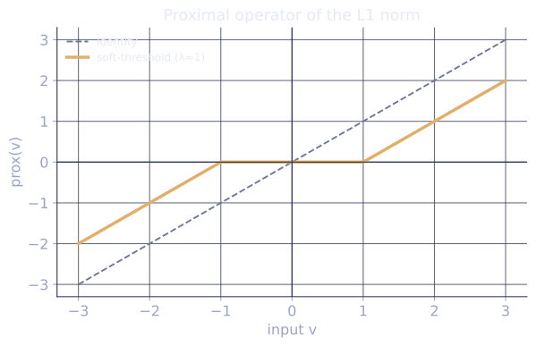
For $g(x) = \lambda \lVert x\rVert_1$ the prox decouples across coordinates, and each solves $\min_{x_i}\lambda|x_i| + \frac{1}{2\eta}(x_i - v_i)^2$ . The solution is the soft-thresholding operator:

\operatorname{prox}_{\eta\lambda\lVert\cdot\rVert_1}(v)_i = \operatorname{sign}(v_i)\,\max(|v_i| - \eta\lambda,\ 0).

It shrinks every coordinate toward zero by $\eta\lambda$ and sets to exactly zero anything smaller than the threshold. This is where L1's sparsity comes from mechanically: the prox step zeroes out small coordinates each iteration. Proximal gradient descent with this prox is ISTA, the iterative soft-thresholding algorithm for LASSO.

Watching the operator act on a few coordinates makes the two behaviors concrete. With threshold $t = \eta\lambda = 0.5$ :

A large coordinate $v = 2.0$ survives but is pulled in: $\operatorname{sign}(2.0)\max(2.0 - 0.5,\,0) = 1.5$ .
A mid coordinate $v = 0.8$ takes the same fixed $0.5$ cut, dropping to $0.3$ . The shrinkage is the same absolute amount, so it bites hardest in relative terms here.
A small coordinate $v = 0.3$ falls below the threshold and is set to $0$ .
The sign carries through unchanged: $v = -1.2$ maps to $-0.7$ , and $v = -0.4$ maps to $0$ .

Contrast this with the gradient step on a smooth L2 penalty, which would scale every coordinate by a factor like $0.9$ : the small $0.3$ would become $0.27$ , still nonzero. Soft-thresholding subtracts a constant instead of scaling, and that constant is what pushes small coordinates to exact zero rather than merely shrinking them.

The proximal operator of the L1 norm is soft-thresholding: it shrinks each coordinate toward zero by λ and clamps small ones exactly to zero, creating sparsity.

Check it on arrays

python · numpy

import numpy as np

rng = np.random.default_rng(0)

# Sparse recovery: y = A x_true + noise, x_true mostly zero (n < d, underdetermined).
n, d, k = 150, 200, 8
A = rng.normal(size=(n, d)) / np.sqrt(n)
x_true = np.zeros(d)
x_true[rng.choice(d, k, replace=False)] = rng.normal(size=k) * 3
y = A @ x_true + 0.01 * rng.normal(size=n)

def soft_threshold(v, t):
    return np.sign(v) * np.maximum(np.abs(v) - t, 0.0)

L = np.linalg.eigvalsh(A.T @ A).max()              # smoothness of 0.5||Ax-y||^2
eta = 1.0 / L
lam = 0.1

x = np.zeros(d)
for _ in range(1500):
    grad = A.T @ (A @ x - y)                       # gradient of the smooth part
    x = soft_threshold(x - eta * grad, eta * lam)  # prox step

print("recovered nonzeros:", int(np.sum(np.abs(x) > 1e-2)), " true:", k)
print("support match:", np.array_equal(np.abs(x) > 1e-2, x_true != 0))
print("reconstruction error:", round(np.linalg.norm(x - x_true), 4))

ISTA recovers the correct sparse support through repeated soft-thresholding, with small coordinates driven to exact zero.

Exercises

Exercise 1. Apply soft-thresholding with threshold $t = \eta\lambda = 0.5$ to the vector $v = (2.0,\, 0.8,\, 0.3,\, -1.2,\, -0.4)$ by hand, coordinate by coordinate.

Solution

Step 1. The operator is $\operatorname{prox}(v)_i = \operatorname{sign}(v_i)\max(|v_i| - 0.5,\, 0)$ . Apply it to each entry.

Step 2. Work through the coordinates:

\begin{aligned} 2.0 &\to \operatorname{sign}(2.0)\max(2.0 - 0.5, 0) = +1.5, \\ 0.8 &\to \max(0.8 - 0.5, 0) = +0.3, \\ 0.3 &\to \max(0.3 - 0.5, 0) = 0, \\ -1.2 &\to \operatorname{sign}(-1.2)\max(1.2 - 0.5, 0) = -0.7, \\ -0.4 &\to \operatorname{sign}(-0.4)\max(0.4 - 0.5, 0) = 0. \end{aligned}

The result is $(1.5,\, 0.3,\, 0,\, -0.7,\, 0)$ . Every surviving coordinate is pulled toward zero by the same $0.5$ , and the two coordinates below the threshold become exactly zero.

Exercise 2. Derive soft-thresholding from the proximal definition. For one coordinate, minimize $\phi(x) = \lambda|x| + \frac{1}{2\eta}(x - v)^2$ over $x \in \mathbb{R}$ and recover the formula. Treat the cases $x > 0$ , $x < 0$ , and $x = 0$ separately, since $|x|$ is nondifferentiable at zero.

Solution

Step 1. Where $x > 0$ , $|x| = x$ is smooth and $\phi'(x) = \lambda + \frac{1}{\eta}(x - v) = 0$ gives $x = v - \eta\lambda$ . This is a valid (positive) solution only when $v > \eta\lambda$ .

Step 2. Where $x < 0$ , $|x| = -x$ and $\phi'(x) = -\lambda + \frac{1}{\eta}(x - v) = 0$ gives $x = v + \eta\lambda$ , valid (negative) only when $v < -\eta\lambda$ .

Step 3. For $-\eta\lambda \le v \le \eta\lambda$ neither branch is feasible, so the minimizer sits at the kink $x = 0$ . The optimality condition there uses the subgradient $\partial|0| = [-1, 1]$ :

0 \in \lambda\,\partial|0| + \tfrac{1}{\eta}(0 - v).

This holds exactly when $|v| \le \eta\lambda$ , confirming $x = 0$ on that interval.

Step 4. Stitch the three cases together:

x^\star = \operatorname{sign}(v)\max(|v| - \eta\lambda,\, 0),

the soft-thresholding operator.

Exercise 3 (code). The prox of the indicator of a convex set is Euclidean projection onto that set. Take the box $C = [-1, 1]^d$ , whose prox is clamping. Implement the projection and verify the defining property of a projection: the projected point is the closest point of $C$ to $v$ , so for any other $u \in C$ , $\lVert v - P(v)\rVert \le \lVert v - u\rVert$ .

Solution

python · numpy

import numpy as np

rng = np.random.default_rng(0)

def project_box(v):
    return np.clip(v, -1.0, 1.0)            # prox of indicator of [-1,1]^d

d = 6
for _ in range(2000):
    v = rng.normal(size=d) * 2.0           # often outside the box
    p = project_box(v)
    # any other point u inside the box is no closer to v than p is
    u = rng.uniform(-1.0, 1.0, size=d)
    assert np.linalg.norm(v - p) <= np.linalg.norm(v - u) + 1e-12

# Projection is idempotent: projecting an in-box point returns it unchanged.
inside = rng.uniform(-1.0, 1.0, size=d)
assert np.allclose(project_box(inside), inside)
print("box projection verified for d =", d)

Clamping returns the nearest box point: each coordinate is moved the least possible amount to satisfy $|x_i| \le 1$ . The inequality confirms it is a genuine Euclidean projection, the prox of the box indicator.

The final A3 lesson optimizes functions with no gradient at all, using a probabilistic surrogate: Bayesian optimization.

References

[1]Parikh, N., & Boyd, S. (2014). "Proximal algorithms". Foundations and Trends in Optimization, 1(3), 127-239. The proximal operator and proximal gradient method (doi:10.1561/2400000003).↩
[2]Beck, A., & Teboulle, M. (2009). "A fast iterative shrinkage-thresholding algorithm for linear inverse problems". SIAM Journal on Imaging Sciences, 2(1), 183-202. ISTA, soft-thresholding, and the accelerated $O(1/t^2)$ FISTA rate (doi:10.1137/080716542).↩