Logistic regression

Linear regression returns a real number; classification needs a probability. Logistic regression keeps the linear predictor but maps it to $[0, 1]$ via the logistic (sigmoid) function. The motivation is the exponential-family machinery from A2: the logistic is the natural inverse link of the Bernoulli.

The model

For binary labels $y_i \in \{0, 1\}$,

Equivalently, the log-odds are linear in the features:

This is the logit link. From the exponential-family lesson, the Bernoulli's natural parameter is the log-odds: the logistic does not just look natural, it falls out of the Bernoulli's algebra[1].

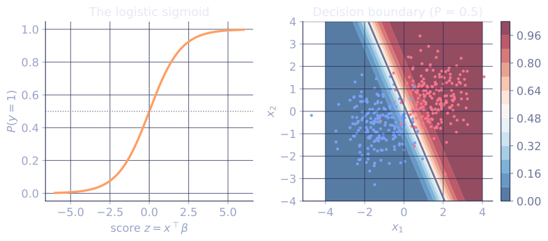
The link runs the whole real line into $[0, 1]$, and a few points fix the scale. A score of $0$ is the decision boundary, $\sigma(0) = 0.5$. A score of $\pm 2$ is already fairly confident ($\sigma(2) \approx 0.88$, $\sigma(-2) \approx 0.12$), and $\pm 4$ is nearly committed ($\sigma(4) \approx 0.982$). The coefficients act on the odds, not the probability: with the code block's $\beta = (-0.5, 1.5, -1.0, 0.7)$, raising feature 1 by one unit adds $1.5$ to the score, which multiplies the odds by $e^{1.5} \approx 4.48$; raising feature 2 by one unit subtracts $1.0$, multiplying the odds by $e^{-1.0} \approx 0.37$. The same coefficient moves the probability by very different amounts depending on where the score starts: near the boundary the sigmoid is steep, out in the tails it is flat.

The log-likelihood

Treat each example as a Bernoulli trial with success probability $p_i = \sigma(x_i^\top\beta)$. The log-likelihood for one example is $y_i \log p_i + (1 - y_i)\log(1 - p_i)$; summing,

Equivalently, since $\log p_i = \log\sigma(x_i^\top\beta)$ simplifies via $\log\sigma(z) = -\log(1 + e^{-z})$,

The negative of $\ell$ is the cross-entropy loss.

Gradient and Hessian

The sigmoid has a clean derivative: $\sigma'(z) = \sigma(z)(1 - \sigma(z))$. Direct computation gives

with $W = \operatorname{diag}(p_i(1 - p_i))$. The Hessian is negative semidefinite, so the log-likelihood is concave: any stationary point is a global maximum. There is no closed form (the gradient equation $X^\top(\mathbf{y} - \sigma(X\beta)) = 0$ is nonlinear in $\beta$), so fitting is iterative.

Newton's method as IRLS

Newton's method applied to maximizing $\ell$:

Rewriting, define the working response $z_i = x_i^\top \beta^{(t)} + (y_i - p_i^{(t)}) / (p_i^{(t)}(1 - p_i^{(t)}))$. Each Newton step is then a weighted least-squares fit $\beta^{(t+1)} = (X^\top W X)^{-1} X^\top W \mathbf{z}$, hence the name iteratively reweighted least squares (IRLS)[2]. Quadratic local convergence, the same as Newton on any smooth convex objective.

For large $n$ or sparse features, plain gradient descent (or its variants from A3) is simpler and often faster per epoch.

Regularization

Adding L2 gives ridge logistic regression: $\ell(\beta) - \frac{\lambda}{2}\lVert\beta\rVert^2$. Adding L1 gives L1 logistic regression for sparse classifiers. Both are MAP under a Gaussian or Laplace prior on $\beta$, and both are fit with the same gradient/proximal machinery as their regression cousins.

Check it on arrays

import numpy as np

rng = np.random.default_rng(0)
n, d = 1000, 4
X = np.column_stack([np.ones(n), rng.normal(size=(n, d - 1))])
beta_true = np.array([-0.5, 1.5, -1.0, 0.7])
p_true = 1 / (1 + np.exp(-X @ beta_true))
y = (rng.random(n) < p_true).astype(float)

def sigmoid(z): return 1 / (1 + np.exp(-z))

def fit_irls(X, y, n_steps=10):
    beta = np.zeros(X.shape[1])
    for _ in range(n_steps):
        p = sigmoid(X @ beta)
        W = p * (1 - p) + 1e-8
        z = X @ beta + (y - p) / W
        beta = np.linalg.solve(X.T @ (W[:, None] * X), X.T @ (W * z))
    return beta

def fit_gd(X, y, lr=0.1, n_steps=2000):
    beta = np.zeros(X.shape[1])
    for _ in range(n_steps):
        p = sigmoid(X @ beta)
        beta += lr * X.T @ (y - p) / len(y)
    return beta

beta_irls = fit_irls(X, y)
beta_gd = fit_gd(X, y)
print("IRLS beta:", np.round(beta_irls, 3))
print("GD   beta:", np.round(beta_gd, 3))
print("true     :", beta_true)

# Predictions
p_hat = sigmoid(X @ beta_irls)
acc = np.mean((p_hat > 0.5) == y)
print(f"accuracy: {acc:.3f}")

# Log-likelihood is concave: Hessian -X^T W X is NSD
W = p_hat * (1 - p_hat)
H = -X.T @ (W[:, None] * X)
print("Hessian eigvals all <= 0:", np.all(np.linalg.eigvalsh(H) <= 1e-10))

IRLS converges in a handful of steps; gradient descent reaches the same solution more slowly; the Hessian's eigenvalues are nonpositive, confirming concavity.

Exercises

Exercise 1. A fitted model has $\beta = (-0.5, 1.5, -1.0, 0.7)$ (the first entry is the intercept). For a feature vector $x = (1, 1, 0, 0)$ (the leading 1 is the intercept term), compute the linear score, the predicted probability $\sigma(x^\top\beta)$, and the odds, by hand.

Exercise 2. Derive the gradient $\nabla\ell = X^\top(\mathbf{y} - \mathbf{p})$ of the log-likelihood, starting from $\ell(\beta) = \sum_i y_i x_i^\top\beta - \log(1 + e^{x_i^\top\beta})$ and using $\sigma'(z) = \sigma(z)(1 - \sigma(z))$.

Exercise 3 (code). The log-likelihood is concave, so it has a unique maximum. Implement the negative log-likelihood and its gradient, then verify the gradient is correct against a finite-difference approximation at a random $\beta$. Confirm the maximum absolute difference is below $10^{-5}$.

import numpy as np

rng = np.random.default_rng(0)
n, d = 200, 4
X = np.column_stack([np.ones(n), rng.normal(size=(n, d - 1))])
beta_true = np.array([-0.5, 1.5, -1.0, 0.7])
p_true = 1 / (1 + np.exp(-X @ beta_true))
y = (rng.random(n) < p_true).astype(float)

def sigmoid(z): return 1 / (1 + np.exp(-z))

def neg_log_lik(beta):
    z = X @ beta
    # log(1 + e^z) computed stably as max(z,0) + log(1 + e^{-|z|})
    log1pexp = np.maximum(z, 0) + np.log1p(np.exp(-np.abs(z)))
    return -np.sum(y * z - log1pexp)

def grad(beta):
    return -X.T @ (y - sigmoid(X @ beta))   # negative of X^T(y - p)

beta0 = rng.normal(size=d)
g_analytic = grad(beta0)

# Central finite differences
eps = 1e-6
g_numeric = np.zeros(d)
for j in range(d):
    step = np.zeros(d); step[j] = eps
    g_numeric[j] = (neg_log_lik(beta0 + step) - neg_log_lik(beta0 - step)) / (2 * eps)

max_diff = np.abs(g_analytic - g_numeric).max()
assert max_diff < 1e-5
print("max |analytic - numeric| gradient:", round(float(max_diff), 9))

The next lesson generalizes to multi-class with the softmax.

References

- [1]Hastie, T., Tibshirani, R., & Friedman, J. (2009). The Elements of Statistical Learning (2nd ed.), §4.4. Springer. doi:10.1007/978-0-387-84858-7. Logistic regression and its log-odds link.↩
- [2]McCullagh, P., & Nelder, J. A. (1989). Generalized Linear Models (2nd ed.), §4.4. Chapman & Hall. IRLS as the standard fitting algorithm.↩