Ridge regression

When the design matrix has nearly collinear columns or more features than examples, OLS coefficients become enormous and unstable. Ridge regression adds an L2 penalty to the loss, trading a small bias for a large variance reduction. The closed form has a clean SVD interpretation: ridge shrinks the small-singular-value directions the most.

The objective

Ridge regression adds an L2 (Tikhonov) penalty to the OLS loss:

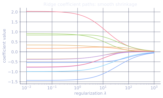
with $\lambda \ge 0$ controlling the shrinkage. At $\lambda = 0$ it is OLS; as $\lambda \to \infty$ all coefficients shrink to zero. The intercept is usually not penalized (center the data instead).

Closed-form solution

Setting the gradient of the objective to zero,

so

The added $\lambda I$ makes $X^\top X + \lambda I$ always invertible (its eigenvalues are shifted up by $\lambda > 0$), which is the cure for the collinearity disease of OLS.

The SVD reading: shrink small directions hardest

Let $X = U \Sigma V^\top$ be the SVD with singular values $\sigma_j$. Substitute:

Compare to OLS: $\hat\beta_{\text{OLS}} = V\,\operatorname{diag}(1/\sigma_j)\,U^\top \mathbf{y}$. The shrinkage factor in direction $j$ is

Directions with large $\sigma_j$ (high variance in $X$, well-determined) are barely shrunk: $\sigma_j^2/(\sigma_j^2 + \lambda) \approx 1$. Directions with small $\sigma_j$ (collinear or rarely seen) get crushed: $\sigma_j^2/(\sigma_j^2 + \lambda) \approx 0$. Ridge does not zero out coefficients; it bends the OLS solution back toward the origin proportionally to how poorly each direction was determined.

Fix $\lambda = 1$ and read the factor across a range of singular values to feel the asymmetry:

• $\sigma_j = 10$ (a well-determined direction): factor $100/101 \approx 0.99$, almost untouched.
• $\sigma_j = 1$ (singular value equal to $\sqrt{\lambda}$): factor $1/2 = 0.5$, the crossover where the coefficient is halved.
• $\sigma_j = 0.1$ (a nearly collinear direction): factor $0.01/1.01 \approx 0.0099$, kept down to about $1\%$ of its OLS value.

The penalty barely sees the strong directions and almost erases the weak ones, which is the point: the weak directions are where OLS blows up.

Ridge as MAP estimation

Place a Gaussian prior $\beta \sim \mathcal{N}(0, \tau^2 I)$ and combine with the Gaussian likelihood from the MLE lesson. The negative log posterior is

Maximizing the posterior (MAP) is the same as ridge with $\lambda = \sigma^2/\tau^2$. Stronger prior belief in small coefficients (small $\tau^2$) means larger $\lambda$. Regularization is a prior in disguise[2].

Bias-variance tradeoff at the lever

Ridge biases coefficients toward zero (the bias term in the bias-variance decomposition grows) but cuts their sensitivity to the data (variance shrinks). On problems where OLS variance is the dominant error term (small $n$, large $d$, collinear features), the net effect of even a small $\lambda$ is a lower expected test error. The optimal $\lambda$ is chosen by cross-validation.

Check it on arrays

import numpy as np

rng = np.random.default_rng(0)
n, d = 30, 12                                # n only slightly > d
X = rng.normal(size=(n, d))
X[:, 0] = 1.0
beta_true = rng.normal(size=d)
y = X @ beta_true + 0.3 * rng.normal(size=n)

def ridge(X, y, lam):
    # Penalize every coefficient EXCEPT the intercept (column 0 is the constant
    # 1). Otherwise large lambda shrinks the intercept toward 0, biasing
    # predictions on uncentered targets.
    d = X.shape[1]
    P = np.eye(d); P[0, 0] = 0.0
    return np.linalg.solve(X.T @ X + lam * P, X.T @ y)

def coef_norm(b): return np.linalg.norm(b)
def train_err(b): return np.mean((y - X @ b)**2)

# Sweep lambda and compare to OLS via the SVD shrinkage factors
print(f"{'lambda':>8}  {'||beta||':>9}  {'train MSE':>10}")
for lam in [0.0, 0.1, 1.0, 10.0, 100.0]:
    b = ridge(X, y, lam)
    print(f"{lam:>8.2f}  {coef_norm(b):>9.4f}  {train_err(b):>10.4f}")

# Confirm the SVD shrinkage formula. The closed form penalizes EVERY direction
# uniformly, so for this check we run a fully-penalized ridge variant.
def ridge_all_penalized(X, y, lam):
    return np.linalg.solve(X.T @ X + lam * np.eye(X.shape[1]), X.T @ y)

U, s, Vt = np.linalg.svd(X, full_matrices=False)
lam = 1.0
b_formula = Vt.T @ (s / (s**2 + lam) * (U.T @ y))
b_direct = ridge_all_penalized(X, y, lam)
print("SVD form == fully-penalized ridge:", np.allclose(b_formula, b_direct))

# Cross-validation to choose lambda
from itertools import islice
def cv_score(lam, k=5):
    idx = rng.permutation(n)
    folds = np.array_split(idx, k)
    errs = []
    for fold in folds:
        train = np.setdiff1d(idx, fold)
        b = ridge(X[train], y[train], lam)
        errs.append(np.mean((y[fold] - X[fold] @ b)**2))
    return np.mean(errs)

lams = np.logspace(-2, 2, 9)
scores = [cv_score(l) for l in lams]
best = lams[int(np.argmin(scores))]
print("best lambda:", round(best, 3))

The coefficient norm shrinks as $\lambda$ grows, train MSE grows (fitting less), the SVD shrinkage formula matches the direct solve to machine precision, and cross-validation picks a finite $\lambda$ where bias and variance balance.

Exercises

Exercise 1. For a single direction with singular value $\sigma = 2$ and penalty $\lambda = 4$, compute the ridge shrinkage factor $\sigma^2/(\sigma^2 + \lambda)$ and state by what fraction the OLS coefficient in that direction is reduced.

Exercise 2. Derive the ridge closed form $\hat\beta_\lambda = (X^\top X + \lambda I)^{-1} X^\top \mathbf{y}$ by setting the gradient of the penalized objective to zero, and explain why $X^\top X + \lambda I$ is always invertible for $\lambda > 0$.

Exercise 3 (code). Verify the MAP equivalence numerically: ridge with penalty $\lambda$ equals the maximum-a-posteriori estimate under a Gaussian prior $\beta \sim \mathcal{N}(0, \tau^2 I)$ and Gaussian likelihood with noise variance $\sigma^2$, where $\lambda = \sigma^2/\tau^2$. Compute the ridge solution for a chosen $(\sigma^2, \tau^2)$ and confirm it matches the direct ridge solve with that $\lambda$.

import numpy as np

rng = np.random.default_rng(0)
n, d = 40, 8
X = rng.normal(size=(n, d))
beta_true = rng.normal(size=d)
sigma2 = 0.25                                  # likelihood noise variance
y = X @ beta_true + np.sqrt(sigma2) * rng.normal(size=n)

tau2 = 2.0                                      # prior variance on beta
lam = sigma2 / tau2                             # the MAP <-> ridge bridge

# Ridge solve with lambda = sigma^2 / tau^2.
beta_ridge = np.linalg.solve(X.T @ X + lam * np.eye(d), X.T @ y)

# MAP: minimize (1/sigma^2)||y - Xb||^2 + (1/tau^2)||b||^2. Multiplying the
# normal equations through by sigma^2 gives exactly the ridge system above.
A = (X.T @ X) / sigma2 + np.eye(d) / tau2
b = (X.T @ y) / sigma2
beta_map = np.linalg.solve(A, b)

print("lambda = sigma^2 / tau^2 =", round(lam, 4))
assert np.allclose(beta_ridge, beta_map)
print("ridge == MAP:", np.allclose(beta_ridge, beta_map))

The next lesson swaps the L2 penalty for L1 and gets sparsity instead of shrinkage.

References

- [1]Hoerl, A. E., & Kennard, R. W. (1970). "Ridge regression: biased estimation for nonorthogonal problems". Technometrics, 12(1), 55-67. doi:10.1080/00401706.1970.10488634↩
- [2]Hastie, T., Tibshirani, R., & Friedman, J. (2009). The Elements of Statistical Learning (2nd ed.), §3.4. Springer. doi:10.1007/978-0-387-84858-7. SVD shrinkage view and the Gaussian-prior (MAP) reading.↩