Bias-variance decomposition

The expected error of a predictor decomposes into three independent terms: how far the average prediction sits from the truth, how much predictions wobble across datasets, and irreducible noise. Almost every regularization, ensembling, and model-selection decision in classical ML reduces to navigating this bias-variance tradeoff.

Setup

A target $y$ is generated by an unknown function plus noise,

A learner trained on a random dataset $\mathcal{D}$ outputs a predictor $\hat f_\mathcal{D}(x)$. Both the training data and $\varepsilon$ are random, so $\hat f_\mathcal{D}(x)$ is also a random variable. Fix a test point $x$ and ask: what is $\mathbb{E}[(y - \hat f_\mathcal{D}(x))^2]$?

The decomposition

Theorem. For squared loss at a fixed test point,[1]

The bias measures how far the average prediction is from the truth. The variance measures how much predictions move around their average across datasets. The noise is intrinsic; no learner can reduce it.

Proof. Let $\bar f(x) = \mathbb{E}_\mathcal{D}[\hat f_\mathcal{D}(x)]$. Expand $y - \hat f_\mathcal{D}$ around the truth and the average:

Square it and take expectations. The three terms are pairwise uncorrelated:

• $\varepsilon$ is independent of $\mathcal{D}$ and has mean zero, so its cross terms vanish.
• $f - \bar f$ is a constant (no randomness), so it commutes with the expectations.
• $\bar f - \hat f_\mathcal{D}$ has mean zero by construction, so its cross terms with the bias also vanish.

Expectations of the three squared terms give noise, bias squared, and variance. $\qquad\blacksquare$

What the terms control

A high-bias estimator misses the true function on average: it is too rigid for the data (linear model fitting a curve). Cutting bias means using a more expressive class.

A high-variance estimator chases the particular training set: it has the expressive power to fit, but the fits are unstable. Cutting variance means averaging across data (bagging), regularizing (ridge, LASSO), or using a simpler model.

The noise floor $\sigma^2$ is the lower bound. Even the best possible predictor cannot beat it.

Where bias-variance shows up

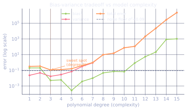
• Polynomial degree. Low-degree polynomials underfit (bias). High-degree polynomials wiggle (variance). The right degree is at the U-shape's minimum.
• k-NN. $k = 1$ has zero training error but enormous variance. Large $k$ smooths over too much detail (bias). The bias-variance lens chooses $k$.
• Trees vs forests. A deep tree has near-zero bias and huge variance. Averaging many decorrelated trees (bagging) kills the variance without introducing bias. This is why random forests work[2].
• Ridge and LASSO. Shrinking coefficients trades a little bias for a large variance reduction, which is the entire point of regularization.

Check it on arrays

The cleanest empirical check: vary model complexity on the same task, repeat training across many random datasets, and watch bias, variance, and total error trace out the canonical U-shape.

import numpy as np

rng = np.random.default_rng(0)

def f(x): return np.sin(2 * np.pi * x)            # ground truth
def gen_dataset(n=30, sigma=0.3, rng=rng):
    x = rng.uniform(0, 1, n)
    return x, f(x) + sigma * rng.normal(size=n)

# Evaluate at a grid of test points
x_test = np.linspace(0, 1, 200)
f_test = f(x_test)

def fit_polynomial(x, y, degree):
    coefs = np.polyfit(x, y, degree)
    return lambda x_eval: np.polyval(coefs, x_eval)

# For each degree, repeat the experiment over many random datasets
degrees = [1, 3, 5, 9, 15]
trials = 200
print("degree  bias^2     variance   total      noise (true 0.09)")
for d in degrees:
    preds = np.zeros((trials, len(x_test)))
    for t in range(trials):
        x_tr, y_tr = gen_dataset(rng=np.random.default_rng(1000 + t))
        preds[t] = fit_polynomial(x_tr, y_tr, d)(x_test)
    mean_pred = preds.mean(axis=0)
    bias2 = np.mean((mean_pred - f_test)**2)
    var = np.mean(preds.var(axis=0))
    sigma2 = 0.3**2
    total = bias2 + var + sigma2
    print(f"  {d:>2}    {bias2:.4f}    {var:.4f}    {total:.4f}   {sigma2:.4f}")

Low degrees show large bias; high degrees show large variance; total error has a U-shape with a minimum at moderate complexity.

Exercises

Exercise 1. A constant predictor ignores $x$ and always outputs a fixed value $c$, so $\hat f_\mathcal{D}(x) = c$ regardless of the data. Identify its bias, variance, and the noise term at a test point where the truth is $f(x)$. What does this say about the extreme low-complexity end of the tradeoff?

Exercise 2. Bagging averages $B$ predictors $\hat f^{(1)}, \dots, \hat f^{(B)}$ trained on independent datasets, outputting $\bar f_B(x) = \frac{1}{B}\sum_b \hat f^{(b)}(x)$. Assuming the $B$ predictors are identically distributed with variance $v$ and pairwise correlation $\rho$, derive the variance of the average and explain why decorrelating the trees (small $\rho$) is what makes random forests work.

Exercise 3 (code). Estimate bias and variance for $k$-nearest-neighbor regression on $f(x) = \sin(2\pi x)$ at the query $x = 0.25$, sweeping $k$. Confirm that 1-NN variance is about $\sigma^2$, that variance falls as $k$ grows, and that the wide window adds bias at this peak of the sine.

import numpy as np

def f(x): return np.sin(2 * np.pi * x)
x_q = 0.25                 # the peak of the sine: wide averaging biases downward
f_q = f(x_q)
sigma = 0.3

def knn_predict(x_tr, y_tr, x_query, k):
    idx = np.argsort(np.abs(x_tr - x_query))[:k]
    return y_tr[idx].mean()

trials = 4000
print(" k    bias^2     variance")
results = {}
for k in [1, 5, 30]:
    preds = np.zeros(trials)
    for t in range(trials):
        r = np.random.default_rng(2000 + t)
        x_tr = r.uniform(0, 1, 80)
        y_tr = f(x_tr) + sigma * r.normal(size=80)
        preds[t] = knn_predict(x_tr, y_tr, x_q, k)
    bias2 = (preds.mean() - f_q) ** 2
    var = preds.var()
    results[k] = (bias2, var)
    print(f"{k:>2}   {bias2:.5f}    {var:.5f}")

assert np.isclose(results[1][1], sigma ** 2, atol=0.02)   # 1-NN variance ~ sigma^2
assert results[30][1] < results[1][1]                     # averaging cuts variance
assert results[30][0] > results[1][0]                     # wide window adds bias

The next lesson uses this lens to motivate ridge regression: shrink the coefficients, accept a small bias, and gain a much larger variance reduction.