LASSO and L1 regularization

Ridge shrinks coefficients but rarely sets them to zero. The LASSO replaces the L2 penalty with L1 and produces sparse solutions: most coefficients are exactly zero. The trick is that the L1 ball has corners, and the loss landscape prefers them; the algorithmic counterpart is soft-thresholding.

The objective

The L1 penalty $\lVert \beta\rVert_1 = \sum_j |\beta_j|$ is convex but not differentiable at zero. There is no closed-form solution in general; the objective is solved iteratively.

Why L1 produces sparsity

Picture the level sets of the squared-error loss as ellipses around $\hat\beta_{\text{OLS}}$, and the constraint region as the L1 ball (a diamond in 2D, with corners on the axes). The constrained minimum is where the smallest ellipse touches the diamond.

The L2 ball is round, so contact is generic, in the interior of a face; ridge shrinks but does not zero. The L1 ball has corners on the axes; the ellipse touches a corner with high probability, and at a corner some coordinates are exactly zero. The corners of L1 are where sparsity is born[2].

Proximal gradient (ISTA)

The L1 part has a closed-form proximal operator: soft-thresholding. For a single coordinate,

which shrinks $v$ toward zero by $\eta\lambda$ and snaps to exactly zero anything smaller than the threshold. The proximal-methods lesson derives this.

Proximal gradient descent (ISTA) alternates a gradient step on the smooth part with a prox step:

The step size $\eta \le n / \sigma_{\max}^2(X)$ ensures convergence. Each iteration is $O(nd)$. Coordinates whose gradient is too small to overcome $\lambda$ are zeroed out and stay zero, giving sparse iterates.

The Bayesian reading

Ridge was MAP under a Gaussian prior. The LASSO is MAP under a Laplace prior $p(\beta_j) \propto \exp(-|\beta_j| / b)$. The Laplace distribution is peaked at zero (which is why MAP prefers exact zeros), where the Gaussian is rounded. Same algorithmic principle, different prior, different geometry.

When LASSO wins, and where it fails

• Sparse truth. If the true model uses only a small subset of features, LASSO recovers their support under incoherence conditions.
• Correlated features. When two columns are highly correlated, LASSO picks one arbitrarily and zeroes the other; elastic net (next lesson) addresses this.
• Grouped features. LASSO selects within groups arbitrarily; the group LASSO penalizes group norms instead.

Check it on arrays

import numpy as np

rng = np.random.default_rng(0)
n, d, k = 150, 200, 8                              # n < d, k true nonzeros
A = rng.normal(size=(n, d)) / np.sqrt(n)
beta_true = np.zeros(d)
beta_true[rng.choice(d, k, replace=False)] = rng.normal(size=k) * 3
y = A @ beta_true + 0.01 * rng.normal(size=n)

def soft_threshold(v, t):
    return np.sign(v) * np.maximum(np.abs(v) - t, 0.0)

def lasso(A, y, lam, steps=2000):
    n = A.shape[0]
    L = np.linalg.eigvalsh(A.T @ A / n).max()
    eta = 1.0 / L
    beta = np.zeros(A.shape[1])
    for _ in range(steps):
        grad = A.T @ (A @ beta - y) / n
        beta = soft_threshold(beta - eta * grad, eta * lam)
    return beta

beta_hat = lasso(A, y, lam=0.1)

nz_recovered = int(np.sum(np.abs(beta_hat) > 1e-2))
print(f"recovered nonzeros: {nz_recovered}  true: {k}")
support_true = beta_true != 0
support_hat = np.abs(beta_hat) > 1e-2
print(f"support match: {np.array_equal(support_hat, support_true)}")
print(f"reconstruction error: {np.linalg.norm(beta_hat - beta_true):.4f}")

# Sweep lambda: more shrinkage -> fewer nonzeros
for lam in [0.05, 0.1, 0.2, 0.5]:
    b = lasso(A, y, lam, steps=1500)
    nz = int(np.sum(np.abs(b) > 1e-2))
    print(f"lambda={lam:.2f}: nonzeros={nz}  ||b - b*||={np.linalg.norm(b - beta_true):.3f}")

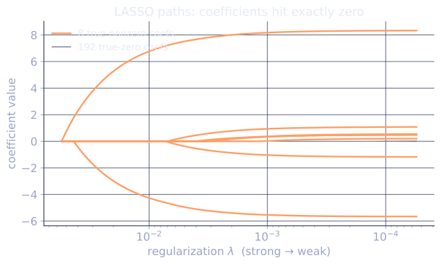
LASSO recovers the true sparse support exactly at moderate $\lambda$; sweeping $\lambda$ traces a path from dense (small $\lambda$) to all-zero (large $\lambda$).

Exercises

Exercise 1. Derive the one-dimensional soft-thresholding rule from scratch. Minimize $g(\beta) = \frac{1}{2}(\beta - v)^2 + \lambda|\beta|$ over $\beta \in \mathbb{R}$ and show the minimizer is $\operatorname{sign}(v)\max(|v| - \lambda, 0)$.

Exercise 2. For an orthonormal design ($X^\top X = I$), show that the full LASSO solution decouples into one soft-threshold per coordinate applied to the OLS estimate: $\hat\beta_j = \operatorname{sign}(\hat\beta_j^{\text{OLS}})\max(|\hat\beta_j^{\text{OLS}}| - \lambda, 0)$. Contrast this with ridge, which only scales each coordinate.

Exercise 3 (code). The soft-thresholding operator is claimed to be the proximal operator of $\lambda|\cdot|$. Verify it numerically: for many random $v$, solve $\arg\min_\beta \frac{1}{2}(\beta - v)^2 + \lambda|\beta|$ by a fine 1D grid search and confirm it matches $\operatorname{soft}(v, \lambda)$, with values inside $[-\lambda, \lambda]$ sent exactly to zero.

import numpy as np

def soft(v, t):
    return np.sign(v) * np.maximum(np.abs(v) - t, 0.0)

rng = np.random.default_rng(0)
lam = 0.4
vs = rng.uniform(-2, 2, 1000)
grid = np.linspace(-3, 3, 60001)        # fine 1D search shared across all v
sol = np.array([grid[np.argmin(0.5 * (grid - v) ** 2 + lam * np.abs(grid))] for v in vs])
closed = soft(vs, lam)

assert np.max(np.abs(sol - closed)) < 1e-3        # grid minimizer matches closed form
small = vs[np.abs(vs) <= lam]
assert np.allclose(soft(small, lam), 0.0)         # within the band -> exactly zero
print("max |grid_min - soft| =", round(float(np.max(np.abs(sol - closed))), 5))

The next lesson combines L1 and L2 to fix LASSO's correlated-feature behavior.

References

- [1]Tibshirani, R. (1996). "Regression shrinkage and selection via the lasso". JRSS-B, 58(1), 267-288. doi:10.1111/j.2517-6161.1996.tb02080.x↩
- [2]Hastie, T., Tibshirani, R., & Friedman, J. (2009). The Elements of Statistical Learning (2nd ed.), §3.4. Springer. doi:10.1007/978-0-387-84858-7. The L1-ball geometry that produces sparsity.↩