Linear regression as maximum likelihood

The previous lesson derived OLS from a geometric loss. The same estimator falls out of a likelihood once you say what the noise distribution is. Under Gaussian noise, OLS is the maximum-likelihood estimator, and the residuals deliver an MLE for the noise variance for free.

The probabilistic model

Replace the loss-only model with a generative assumption: targets are noisy linear functions of features,

with independent errors across examples. The unknowns are now $\beta$ and the noise variance $\sigma^2$.

The likelihood

The Gaussian PDF gives the likelihood of each observation:

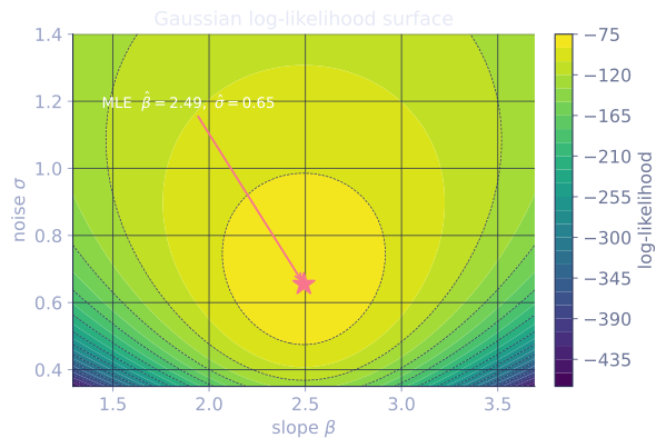
By independence, the joint log-likelihood is

MLE for $\beta$: same as OLS

The only $\beta$-dependent term is the sum of squared residuals, with a negative sign and positive scalar prefactor. Maximizing $\ell$ in $\beta$ is the same as minimizing the sum of squared residuals:

The OLS estimator is the MLE under Gaussian noise. This is why squared-error loss is the default for regression: it is the negative log-likelihood of a Gaussian, the noise model nothing else has a reason to disagree with by default.

MLE for $\sigma^2$

Substitute $\hat\beta$ back into $\ell$ and differentiate with respect to $\sigma^2$. Setting the derivative to zero,

where $r_i = y_i - x_i^\top\hat\beta$ are the residuals. The MLE for noise variance is the mean squared residual. The unbiased estimator divides by $n - d$ instead of $n$ (the same correction that turned sample-variance into $n - 1$ for a single sample):

The $n - d$ correction accounts for the degrees of freedom lost to fitting $d$ coefficients. The two estimators differ by the factor $(n - d)/n$, which is the fraction by which the MLE underestimates on average, so the gap is a story about sample size. Fitting $d = 3$ coefficients:

• $n = 10$: factor $7/10 = 0.7$, the MLE runs about $30\%$ low. With ten points and three coefficients, three of the residuals are nearly forced to zero, and dividing by $n$ ignores that.
• $n = 50$: factor $47/50 = 0.94$, a $6\%$ underestimate.
• $n = 500$ (the code block's size): factor $497/500 \approx 0.994$, under $1\%$. The correction barely moves the answer here, which is why the two printed variances come out close.

The correction matters when $d$ is a real fraction of $n$ and is negligible when $n \gg d$.

Why this matters

Having the likelihood gives you, in addition to point estimates:

• Confidence intervals on each $\hat\beta_j$ via the Fisher information, which for linear regression equals $\sigma^2 (X^\top X)^{-1}$[2].
• Hypothesis tests (t-tests for individual coefficients, F-tests for groups).
• Model comparison via likelihood-ratio tests and information criteria (AIC, BIC).
• The bridge to ridge regression as MAP under a Gaussian prior on $\beta$, and to LASSO as MAP under a Laplace prior.

Check it on arrays

import numpy as np

rng = np.random.default_rng(1)
n, d = 500, 3
X = np.column_stack([np.ones(n), rng.normal(size=(n, d - 1))])
beta_true = np.array([1.0, 2.5, -0.8])
sigma_true = 0.7
y = X @ beta_true + sigma_true * rng.normal(size=n)

# MLE for beta = OLS
beta_hat = np.linalg.lstsq(X, y, rcond=None)[0]
print("beta_hat:", np.round(beta_hat, 3), " true:", beta_true)

# MLE vs unbiased noise variance
r = y - X @ beta_hat
sigma2_mle = np.mean(r**2)
sigma2_unbiased = np.sum(r**2) / (n - d)
print(f"sigma^2 MLE      = {sigma2_mle:.4f}")
print(f"sigma^2 unbiased = {sigma2_unbiased:.4f}")
print(f"true sigma^2     = {sigma_true**2:.4f}")

# Coefficient standard errors via Fisher info
cov_beta = sigma2_unbiased * np.linalg.inv(X.T @ X)
se = np.sqrt(np.diag(cov_beta))
print("std errors:", np.round(se, 4))
for j, (b, s, bt) in enumerate(zip(beta_hat, se, beta_true)):
    lo, hi = b - 1.96 * s, b + 1.96 * s
    inside = lo <= bt <= hi
    print(f"  beta_{j}: 95% CI [{lo:.3f}, {hi:.3f}] contains truth? {inside}")

The MLE for $\beta$ recovers the OLS estimate, the MLE noise variance is slightly biased low (the unbiased version with $n - d$ is closer to truth), and the 95% confidence intervals from the Fisher information cover the true coefficients.

Exercises

Exercise 1. A single feature-free model fits a constant: $y_i \sim \mathcal{N}(\mu, \sigma^2)$, so $X$ is the all-ones column and $\beta = \mu$. Show that the MLE is the sample mean $\hat\mu = \frac{1}{n}\sum_i y_i$ by differentiating the log-likelihood.

Exercise 2. Prove the residuals are orthogonal to every column of $X$: $X^\top r = 0$ at $\hat\beta_{\text{MLE}}$, where $r = \mathbf{y} - X\hat\beta$. Use this to explain why fitting $d$ coefficients forces the residual vector into an $(n - d)$-dimensional subspace, the degrees-of-freedom story behind the $n - d$ divisor.

Exercise 3 (code). Confirm the $\hat\sigma^2_{\text{MLE}}$ bias factor $(n - d)/n$ empirically. Fit OLS with $d = 4$ coefficients over many random datasets for several sample sizes, and check that the average of $\hat\sigma^2_{\text{MLE}} / \sigma^2$ matches $(n - d)/n$.

import numpy as np

d = 4
sigma2 = 1.5
print("n      mean(MLE)/true   expected (n-d)/n")
for n in [8, 20, 100, 1000]:
    ratios = []
    for t in range(2000):
        r = np.random.default_rng(1000 + t)
        X = np.column_stack([np.ones(n)] + [r.normal(size=n) for _ in range(d - 1)])
        beta = r.normal(size=d)
        y = X @ beta + np.sqrt(sigma2) * r.normal(size=n)
        bhat = np.linalg.lstsq(X, y, rcond=None)[0]
        res = y - X @ bhat
        ratios.append(np.mean(res**2) / sigma2)
    mean_ratio = float(np.mean(ratios))
    expected = (n - d) / n
    print(f"{n:>5}  {mean_ratio:.4f}          {expected:.4f}")
    assert np.isclose(mean_ratio, expected, atol=0.02)

The next lesson tackles the universal tradeoff every estimator faces: bias and variance.

References

- [1]Bishop, C. M. (2006). Pattern Recognition and Machine Learning, §3.1. Springer. Least squares as Gaussian maximum likelihood.↩
- [2]Hastie, T., Tibshirani, R., & Friedman, J. (2009). The Elements of Statistical Learning (2nd ed.), §3.2. Springer. doi:10.1007/978-0-387-84858-7. Sampling distribution and inference for the coefficients.↩