Softmax regression

Logistic regression handles two classes. For $K > 2$ classes, the natural generalization parameterizes one linear score per class and normalizes with the softmax. Training minimizes cross-entropy, which (as the kl-cross-entropy lesson shows) is maximum likelihood under the categorical distribution.

The model

For an input $x \in \mathbb{R}^d$ and $K$ classes, the model has a coefficient vector $\beta_k \in \mathbb{R}^d$ per class. The class probabilities are

The denominator normalizes the scores into a probability distribution ($\sum_k p_k = 1$, every $p_k \ge 0$). This is the softmax of the score vector $z = (x^\top \beta_1, \dots, x^\top \beta_K)$[1].

The model is overparameterized: adding a constant $c$ to every $\beta_k$ leaves the probabilities unchanged. A common fix is to set $\beta_K = 0$ (reduces to logistic regression when $K = 2$); production code keeps all $K$ parameter vectors and lets regularization tie down the redundancy.

Cross-entropy loss

With one-hot true labels $\mathbf{y}_i \in \{e_1, \dots, e_K\}$, the negative log-likelihood per example is the cross-entropy:

The log-sum-exp form is exactly the stable softmax of the numerical-methods lesson; production code always shifts by the maximum before exponentiating.

A few score vectors over three classes make the scale concrete (true class is class 0 throughout, so the per-example loss is $-\log p_0$):

• Confident and right. Scores $(4, 1, 0)$ softmax to $(0.936, 0.047, 0.017)$. The model puts $94\%$ on the true class, paying loss $-\log 0.936 = 0.066$ nats.
• Hesitant. Scores $(1, 0.5, 0)$ give $(0.506, 0.307, 0.186)$: a bare majority on the true class, loss $-\log 0.506 = 0.68$ nats, ten times the confident case.
• No opinion. Scores $(0, 0, 0)$ give the uniform $(0.333, 0.333, 0.333)$, loss $-\log \tfrac13 = 1.099$ nats, the most a three-class model can pay while still ranking the truth first.

The overparameterization from the model section shows up here as shift invariance: adding $10$ to every score, $(14, 11, 10)$, leaves the softmax at $(0.936, 0.047, 0.017)$ unchanged, since the shared constant cancels in the ratio. Only the differences between scores carry information.

Gradient

The gradient with respect to $\beta_k$ has a clean form:

the data residual between predicted probability and the true-class indicator, weighted by features[2]. The objective is convex (the Hessian is again of the form $X^\top W X$ with $W$ positive semidefinite block matrix), so any local minimum is global.

Multi-class metrics shift

Predictions are now distributions over $K$ classes. The classification choice is $\arg\max_k p_k$. Probability quality (calibration, log-loss) becomes the right metric when downstream code consumes probabilities; classification accuracy alone hides miscalibration.

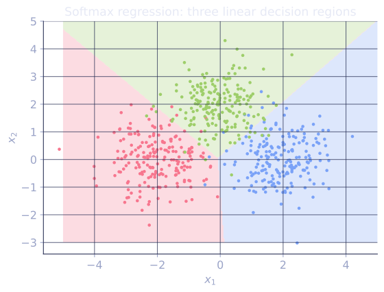
Check it on arrays

import numpy as np

rng = np.random.default_rng(0)

# Synthetic 3-class problem
n_per_class, d = 200, 3
X = np.vstack([
    rng.normal(loc=[2, 0], size=(n_per_class, 2)),
    rng.normal(loc=[-2, 0], size=(n_per_class, 2)),
    rng.normal(loc=[0, 2], size=(n_per_class, 2)),
])
X = np.column_stack([np.ones(len(X)), X])              # intercept
y = np.array([0] * n_per_class + [1] * n_per_class + [2] * n_per_class)
K = 3

def softmax(Z):
    Z = Z - Z.max(axis=1, keepdims=True)              # stable shift
    e = np.exp(Z)
    return e / e.sum(axis=1, keepdims=True)

def fit(X, y, K, lr=0.5, steps=2000, lam=0.0):
    n, d = X.shape
    Y = np.eye(K)[y]                                  # one-hot
    B = np.zeros((d, K))
    for _ in range(steps):
        P = softmax(X @ B)
        grad = X.T @ (P - Y) / n + lam * B
        B -= lr * grad
    return B

B = fit(X, y, K, lr=1.0, steps=3000)

P = softmax(X @ B)
y_pred = P.argmax(axis=1)
acc = np.mean(y_pred == y)
log_loss = -np.mean(np.log(P[np.arange(len(y)), y] + 1e-12))
print(f"accuracy: {acc:.3f}")
print(f"log loss: {log_loss:.3f}")

# Sanity check: probabilities are valid
print(f"row sums (should be 1): {P.sum(axis=1)[:3]}")
print(f"all positive: {(P > 0).all()}")

# When K=2, softmax reduces to logistic on the difference of scores
B_binary = fit(X[:2 * n_per_class], y[:2 * n_per_class], K=2, lr=1.0)
diff = X[:2 * n_per_class] @ (B_binary[:, 1] - B_binary[:, 0])
p1 = 1 / (1 + np.exp(-diff))
print("softmax K=2 matches logistic:", np.allclose(p1, softmax(X[:2 * n_per_class] @ B_binary)[:, 1], atol=1e-6))

The classifier gets the three Gaussian blobs apart, probabilities normalize per row, and the binary case reduces to logistic on the score difference.

Exercises

Exercise 1. Compute the softmax of the score vector $z = (2, 1, 0)$ over three classes by hand, then give the cross-entropy loss in nats if the true class is class 0.

Exercise 2. Prove the shift invariance of the softmax: adding the same constant $c$ to every score leaves the output probabilities unchanged. This is why only differences between scores carry information.

Exercise 3 (code). Implement softmax cross-entropy and its gradient with respect to the scores $Z$. For one-hot labels the gradient is $P - Y$ (predicted probabilities minus the one-hot targets). Verify this gradient against a finite-difference check on the total loss, and confirm the max difference is below $10^{-6}$.

import numpy as np

rng = np.random.default_rng(0)
n, K = 12, 4
Z = rng.normal(size=(n, K))                    # raw scores
y = rng.integers(0, K, size=n)
Y = np.eye(K)[y]                               # one-hot targets

def softmax(Z):
    Z = Z - Z.max(axis=1, keepdims=True)
    e = np.exp(Z)
    return e / e.sum(axis=1, keepdims=True)

def loss(Z):
    P = softmax(Z)
    return -np.sum(Y * np.log(P + 1e-12))

P = softmax(Z)
grad_analytic = P - Y                           # d loss / d Z

# Finite-difference check on every entry of Z.
eps = 1e-6
grad_numeric = np.zeros_like(Z)
for i in range(n):
    for k in range(K):
        Zp = Z.copy(); Zp[i, k] += eps
        Zm = Z.copy(); Zm[i, k] -= eps
        grad_numeric[i, k] = (loss(Zp) - loss(Zm)) / (2 * eps)

max_diff = np.abs(grad_analytic - grad_numeric).max()
assert max_diff < 1e-6
print("max |analytic - numeric| gradient:", round(float(max_diff), 9))

The next lesson zooms out to the general framework that unifies linear, logistic, and Poisson regression: GLMs.

References

- [1]Bishop, C. M. (2006). Pattern Recognition and Machine Learning, §4.3.4. Springer. Softmax (multinomial logistic) regression.↩
- [2]Hastie, T., Tibshirani, R., & Friedman, J. (2009). The Elements of Statistical Learning (2nd ed.), §4.4. Springer. doi:10.1007/978-0-387-84858-7. Multiclass logistic regression and its gradient.↩