Linear regression and OLS

Linear regression is the simplest supervised learner: model a target as a linear function of features plus noise, and fit the coefficients to minimize squared error. The closed form falls out of the least-squares lesson, but interpreting it as a projection is what makes the rest of the curriculum (ridge, LASSO, GLMs, calibration) click into place.

The model

Given $n$ examples with feature vectors $x_i \in \mathbb{R}^d$ and targets $y_i \in \mathbb{R}$, the linear regression model assumes

where $\beta \in \mathbb{R}^d$ are the unknown coefficients and $\varepsilon_i$ is zero-mean noise. Stacking rows, write $X \in \mathbb{R}^{n \times d}$ for the design matrix and $\mathbf{y} \in \mathbb{R}^n$ for the target vector; the model is

A column of ones in $X$ absorbs the intercept, so the formulas below cover the intercept case without extra notation.

The OLS objective

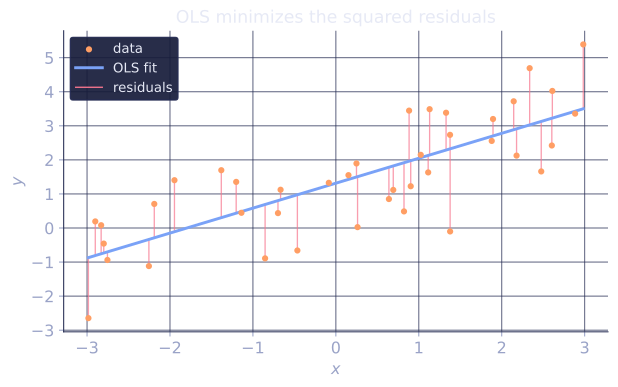
Ordinary least squares (OLS) picks the coefficients that minimize the sum of squared residuals:

Squared error is convex in $\beta$ (Hessian $2X^\top X \succeq 0$), so the minimum is wherever the gradient vanishes.

The normal equations

Differentiating with respect to $\beta$ using matrix calculus,

Setting it to zero gives the normal equations

When $X$ has full column rank, $X^\top X$ is invertible and

If columns of $X$ are collinear, $X^\top X$ is singular and the minimizer is not unique; that is the gap ridge regression will close.

Geometric reading: projection onto the column space

The fitted values are $\hat{\mathbf{y}} = X\hat\beta$. Substituting,

where $P = X(X^\top X)^{-1}X^\top$ is the projection matrix onto the column space of $X$ (idempotent, $P^2 = P$, and symmetric)[2]. The residual $\mathbf{r} = \mathbf{y} - \hat{\mathbf{y}}$ lives in the orthogonal complement: $X^\top \mathbf{r} = 0$ (this is exactly the normal equations rewritten).

The geometric picture: $\hat{\mathbf{y}}$ is the closest point in $\operatorname{col}(X)$ to $\mathbf{y}$, and OLS is least-squares projection. The whole rest of the lesson chain is a refinement of this picture.

Numerical route

Forming $X^\top X$ squares the condition number; the conditioning lesson explains why. The numerically stable route uses the QR factorization $X = QR$:

solved by back-substitution. Production code uses QR (numpy's lstsq) or the SVD, not the explicit inverse.

Check it on arrays

import numpy as np

rng = np.random.default_rng(0)
n, d = 200, 4
X = rng.normal(size=(n, d))
X[:, 0] = 1.0                                  # intercept
beta_true = np.array([2.0, -1.5, 0.7, 0.3])
y = X @ beta_true + 0.2 * rng.normal(size=n)

# Closed form via the normal equations
beta_normal = np.linalg.solve(X.T @ X, X.T @ y)
print("normal-eq beta:", np.round(beta_normal, 4))

# Stable route: QR factorization
Q, R = np.linalg.qr(X)
beta_qr = np.linalg.solve(R, Q.T @ y)
print("QR beta:       ", np.round(beta_qr, 4))

# Reference: numpy's least-squares solver (SVD-based)
beta_lstsq, *_ = np.linalg.lstsq(X, y, rcond=None)
print("lstsq beta:    ", np.round(beta_lstsq, 4))
print("agree?", np.allclose(beta_qr, beta_lstsq))

# Residuals are orthogonal to every column of X
y_hat = X @ beta_qr
r = y - y_hat
print("X^T r (should be ~0):", np.round(X.T @ r, 6))

# Projection matrix: P y == y_hat, and P^2 == P
P = X @ np.linalg.solve(X.T @ X, X.T)
print("P y == y_hat:", np.allclose(P @ y, y_hat))
print("P^2 == P:    ", np.allclose(P @ P, P, atol=1e-10))

The three routes recover the same $\hat\beta$, the residual is numerically orthogonal to every feature column, and $P$ is idempotent.

Exercises

Exercise 1. Fit OLS by hand for a single feature with no intercept. Given the three points $(x, y) = (1, 2), (2, 2), (3, 4)$ and the model $y = \beta x$ (scalar $\beta$, design matrix $X = (1, 2, 3)^\top$), solve the normal equation $X^\top X\,\hat\beta = X^\top \mathbf{y}$ for $\hat\beta$.

Exercise 2. Prove that the OLS residual $\mathbf{r} = \mathbf{y} - X\hat\beta$ is orthogonal to the column space of $X$, i.e. $X^\top \mathbf{r} = 0$, directly from the normal equations.

Exercise 3 (code). A rank-deficient $X$ breaks the explicit inverse but not the SVD-based solver. Build a design matrix whose third column is an exact copy of its second, then show that np.linalg.solve(X.T @ X, ...) fails (singular matrix) while np.linalg.lstsq still returns a valid least-squares fit, and verify that its residual is orthogonal to the columns of $X$.

import numpy as np

rng = np.random.default_rng(0)
n = 50
X = rng.normal(size=(n, 3))
X[:, 2] = X[:, 1]                          # column 3 duplicates column 2: rank 2
beta_true = np.array([1.0, 2.0, -0.5])
y = X @ beta_true + 0.1 * rng.normal(size=n)

# Explicit normal-equation solve fails: X^T X is singular.
singular = False
try:
    np.linalg.solve(X.T @ X, X.T @ y)
except np.linalg.LinAlgError:
    singular = True
assert singular                            # X^T X is not invertible

# lstsq (SVD) returns the minimum-norm least-squares solution regardless.
beta_hat, *_ = np.linalg.lstsq(X, y, rcond=None)
r = y - X @ beta_hat
assert np.allclose(X.T @ r, 0.0, atol=1e-8)   # residual still orthogonal
print("residual orthogonal, max |X^T r| =", round(np.abs(X.T @ r).max(), 10))

The next lesson asks where this estimator comes from probabilistically: it is the MLE under Gaussian noise.

References

- [1]Hastie, T., Tibshirani, R., & Friedman, J. (2009). The Elements of Statistical Learning (2nd ed.), §3.2. Springer. doi:10.1007/978-0-387-84858-7↩
- [2]James, G., Witten, D., Hastie, T., & Tibshirani, R. (2021). An Introduction to Statistical Learning (2nd ed.), §3.1. Springer. The projection/geometry reading of least squares.↩