Poisson and Gamma GLMs

The GLM framework opens up two regression flavors that Gaussian linear regression handles badly: counts (Poisson) and positive continuous durations (Gamma). Both use a log link so the predicted mean stays positive, and both have a variance structure tied to the mean.

Poisson regression for counts

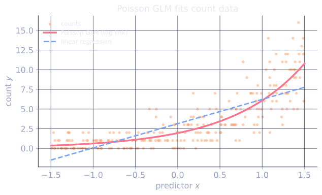
When the response $y$ is a count (number of events in a time window, clicks per session, citations per paper), the Gaussian model is wrong on two grounds: counts are nonnegative integers, and their variance grows with the mean. The Poisson model handles both.

Setup:

• Random component: $y_i \mid x_i \sim \text{Pois}(\mu_i)$, so $\mathbb{E}[y] = \operatorname{Var}(y) = \mu$.
• Link: log link, $\log \mu_i = x_i^\top \beta$, hence $\mu_i = e^{x_i^\top\beta}$.

The log link guarantees the mean stays positive. Coefficients are multiplicative effects on the rate: $e^{\beta_j}$ is the factor by which the expected count multiplies when $x_j$ increases by one unit[1].

Log-likelihood:

Concave in $\beta$. The MLE has no closed form; IRLS converges quickly with $W = \operatorname{diag}(\mu_i)$ and working response $z_i = x_i^\top\beta + (y_i - \mu_i)/\mu_i$.

Overdispersion

The Poisson assumes $\operatorname{Var}(y) = \mu$. Real count data often has variance larger than the mean (overdispersion), because individual rates themselves vary across units. Two standard remedies:

• Quasi-Poisson: scale the variance by a dispersion parameter $\phi$ estimated from residuals, $\operatorname{Var}(y) = \phi\mu$. The point estimates are the same as Poisson; the standard errors widen.
• Negative Binomial: a Poisson-gamma mixture where each unit has its own rate drawn from a Gamma distribution, allowing $\operatorname{Var}(y) = \mu + \mu^2/k$[2].

A back-of-envelope check: if the sample variance of $y$ is much larger than the sample mean, expect overdispersion.

Gamma regression for positive continuous responses

When $y > 0$ is a continuous duration or amount (waiting time, insurance claim, network latency), the Gaussian linear model can predict negative means and assumes constant variance. The Gamma GLM handles both.

Setup:

• Random component: $y_i \mid x_i \sim \text{Gamma}(\text{mean } \mu_i,\ \text{shape } \alpha)$. The variance grows as $\operatorname{Var}(y) = \mu^2/\alpha$, so the coefficient of variation is constant.
• Link: usually log link $\log \mu = x^\top \beta$ in practice (canonical is the reciprocal $1/\mu$, but the log link is preferred because it cannot produce negative means).

Like Poisson, coefficients are multiplicative effects on the mean. The shape parameter $\alpha$ is estimated from the data (or set by the user).

How to choose

A short decision guide:

• $y$ is a count, $\operatorname{Var}(y) \approx \mu$: Poisson.
• $y$ is a count, $\operatorname{Var}(y) > \mu$: Negative Binomial.
• $y > 0$ is continuous with constant coefficient of variation: Gamma.
• $y > 0$ is continuous with constant variance: linear regression on $\log y$ is the lazy alternative.

Check it on arrays

import numpy as np

rng = np.random.default_rng(0)

# Poisson regression on simulated counts
n, d = 500, 3
X = np.column_stack([np.ones(n), rng.normal(size=(n, d - 1))])
beta_true = np.array([0.5, 0.4, -0.3])
mu_true = np.exp(X @ beta_true)
y = rng.poisson(mu_true)

def fit_glm_log(X, y, var_fn, steps=20):
    """IRLS with log link."""
    mu = (y + 1.0).astype(float)
    for _ in range(steps):
        eta = np.log(mu)
        z = eta + (y - mu) / mu                       # canonical-link work resp
        W = mu**2 / var_fn(mu)                        # for log link: W = mu^2/Var(y)
        beta = np.linalg.solve(X.T @ (W[:, None] * X), X.T @ (W * z))
        mu = np.exp(X @ beta)
    return beta, mu

beta_pois, mu_pois = fit_glm_log(X, y, var_fn=lambda m: m)
print("Poisson coefficients:", np.round(beta_pois, 3), " (true ", beta_true, ")")

# Multiplicative interpretation: e^beta gives the rate multiplier
for j, b in enumerate(beta_pois):
    print(f"  e^beta_{j} = {np.exp(b):.3f}  -> rate multiplies by this per +1 unit")

# Gamma regression on positive continuous response with log link
beta_g_true = np.array([1.0, 0.5, -0.2])
mu_g_true = np.exp(X @ beta_g_true)
shape = 4.0
scale = mu_g_true / shape                              # so that mean = shape * scale = mu_g_true
y_g = rng.gamma(shape=shape, scale=scale)

beta_gamma, mu_gamma = fit_glm_log(X, y_g, var_fn=lambda m: m**2 / shape)
print("\nGamma coefficients:  ", np.round(beta_gamma, 3), " (true ", beta_g_true, ")")

# Check overdispersion: Poisson has Var(y) = mu
print(f"\nempirical Var/mean for Poisson data: {y.var() / y.mean():.2f}  (Poisson = 1)")

Both GLMs recover their true coefficients, the multiplicative interpretation of $e^\beta$ holds for the log link, and the Poisson sample variance is close to the sample mean.

Exercises

Exercise 1. A Poisson regression for daily store visits fits intercept $\beta_0 = 2.0$ and a "weekend" coefficient $\beta_1 = 0.7$ (with $x_1 = 1$ on weekends, $0$ otherwise). Compute the expected count on a weekday and on a weekend, and state the multiplicative effect of the weekend.

Exercise 2. Show that the Poisson log-likelihood $\ell(\beta) = \sum_i \big(y_i x_i^\top\beta - e^{x_i^\top\beta} - \log y_i!\big)$ is concave in $\beta$, so any stationary point is the global maximum.

Exercise 3 (code). Overdispersion is the signature that count data violates the Poisson mean-equals-variance assumption. Simulate a negative-binomial-like process (a Poisson whose rate is itself Gamma-distributed across units) and compare its variance-to-mean ratio against a plain Poisson sample with the same mean. Assert the mixed process is overdispersed (ratio above 1.5) while the plain Poisson sits near 1.

import numpy as np

rng = np.random.default_rng(0)
n = 200_000
mean_rate = 5.0

# Plain Poisson: Var/mean should be ~1.
y_pois = rng.poisson(mean_rate, size=n)
ratio_pois = y_pois.var() / y_pois.mean()

# Poisson-Gamma mixture: each unit's rate is Gamma with mean mean_rate.
# This is the negative-binomial construction; it inflates the variance.
shape = 1.0
rates = rng.gamma(shape=shape, scale=mean_rate / shape, size=n)
y_mix = rng.poisson(rates)
ratio_mix = y_mix.var() / y_mix.mean()

print(f"plain Poisson Var/mean: {ratio_pois:.3f}")
print(f"Poisson-Gamma Var/mean: {ratio_mix:.3f}")

assert abs(ratio_pois - 1.0) < 0.05        # Poisson: variance equals mean
assert ratio_mix > 1.5                     # mixture is overdispersed

This closes the C1 linear-models track; the next subsection turns to a different geometric story: max-margin classifiers and kernels.

References

- [1]McCullagh, P., & Nelder, J. A. (1989). Generalized Linear Models (2nd ed.), §6 (Poisson), §8 (Gamma). Chapman & Hall.↩
- [2]Nelder, J. A., & Wedderburn, R. W. M. (1972). "Generalized linear models". JRSS-A, 135(3), 370-384. doi:10.2307/2344614. The original GLM treatment of Poisson and Gamma responses.↩