Least squares & the Moore–Penrose pseudo-inverse

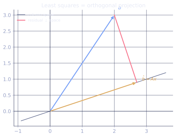
Most real systems are overdetermined: more equations than unknowns, and no exact solution exists. The least-squares criterion picks the $x$ that makes $Ax$ as close to $b$ as possible, and the geometry is a projection.

The least-squares problem

Given $A \in \mathbb{R}^{m \times n}$ with $m > n$ and $b \in \mathbb{R}^m$, find

The objective $\lVert Ax - b\rVert^2$ is a quadratic in $x$ (it opens up: $A^\top A$ is PSD). Its minimum is where the gradient is zero.

Derivation via the gradient

Expand:

Taking the gradient with respect to $x$ and setting it to zero:

giving the normal equations:[1]

If $A$ has full column rank ($n$), $A^\top A$ is invertible, and the unique solution is $\hat{x} = (A^\top A)^{-1} A^\top b$.

Geometric interpretation

$A\hat{x}$ is the projection of $b$ onto $\operatorname{col}(A)$: it is the point in the column space closest to $b$. The residual $r = b - A\hat{x}$ is orthogonal to every column of $A$:

which is exactly the normal equations rewritten. The projection matrix onto $\operatorname{col}(A)$ is

Any symmetric idempotent matrix is a projection; these two properties characterize projections completely.

Numerical route: QR is preferable

Forming $A^\top A$ squares the condition number: $\kappa(A^\top A) = \kappa(A)^2$. The QR route avoids this. Write $A = QR$ (thin QR, $Q \in \mathbb{R}^{m \times n}$, $R \in \mathbb{R}^{n \times n}$ upper triangular). The normal equations become

a triangular system solved by backward substitution.

The Moore–Penrose pseudo-inverse

When $A$ does not have full column rank, the normal equations have infinitely many solutions. The minimum-norm solution (smallest $\lVert x\rVert_2$ among all minimizers of $\lVert Ax - b\rVert_2$) is given by the Moore–Penrose pseudo-inverse $A^+$[2]:

Construction from SVD. Let $A = U\Sigma V^\top$ with rank $r$. Define

where $\Sigma^+$ replaces each nonzero singular value $\sigma_i$ by $1/\sigma_i$ and leaves zeros alone.

Properties:

• If $A$ has full column rank: $A^+ = (A^\top A)^{-1}A^\top$ (the standard formula).
• If $A$ has full row rank: $A^+ = A^\top(AA^\top)^{-1}$ (a right inverse).
• $A A^+ A = A$, $A^+ A A^+ = A^+$, and both $A A^+$ and $A^+ A$ are symmetric.

Check it on arrays

import numpy as np

rng = np.random.default_rng(7)

m, n = 50, 5
A = rng.normal(size=(m, n))
b = rng.normal(size=m)

# Normal equations (full column rank here)
ATA = A.T @ A
ATb = A.T @ b
x_normal = np.linalg.solve(ATA, ATb)

# QR route (numerically preferable)
Q, R = np.linalg.qr(A)
x_qr = np.linalg.solve(R, Q.T @ b)

# Built-in lstsq (uses SVD internally)
x_lstsq, _, _, _ = np.linalg.lstsq(A, b, rcond=None)

print("normal eq residual:", np.linalg.norm(A @ x_normal - b))
print("QR residual:", np.linalg.norm(A @ x_qr - b))
print("lstsq residual:", np.linalg.norm(A @ x_lstsq - b))   # same
print("solutions agree:", np.allclose(x_qr, x_lstsq, atol=1e-10))

# Pseudo-inverse via SVD: also handles rank-deficient A
U, s, Vt = np.linalg.svd(A, full_matrices=False)
A_plus = Vt.T @ np.diag(1.0 / s) @ U.T
x_pinv = A_plus @ b
print("pinv agrees with lstsq:", np.allclose(x_pinv, x_lstsq, atol=1e-10))

# Residual is orthogonal to col(A):
r = b - A @ x_lstsq
print("A^T r (should be ~0):", np.round(A.T @ r, 8))

All four routes agree on the solution; the residual is orthogonal to every column of $A$.

Exercises

Exercise 1. Solve the least-squares problem with $A = \begin{pmatrix} 1 \\ 1 \\ 1 \end{pmatrix}$ and $b = \begin{pmatrix} 2 \\ 4 \\ 6 \end{pmatrix}$ by the normal equations, and state what the scalar $\hat{x}$ represents geometrically.

Exercise 2. Show directly from the definition that the projection matrix $P = A(A^\top A)^{-1}A^\top$ (with $A$ of full column rank) is idempotent ($P^2 = P$) and symmetric ($P^\top = P$).

Exercise 3 (code). Build a rank-deficient $A$ (repeat a column so the column rank is below the number of columns). The normal equations are then singular. Verify that the SVD pseudo-inverse $A^+ b$ still returns a least-squares solution and that, among all minimizers, it has the smallest $\ell^2$ norm.

import numpy as np

rng = np.random.default_rng(3)
m = 30
c = rng.normal(size=m)
A = np.column_stack([c, 2 * c, rng.normal(size=m)])   # col 2 = 2*col 1: rank 2
b = rng.normal(size=m)

# Pseudo-inverse via SVD (drops the zero singular value).
U, s, Vt = np.linalg.svd(A, full_matrices=False)
tol = 1e-10
s_inv = np.where(s > tol, 1.0 / s, 0.0)
A_plus = Vt.T @ np.diag(s_inv) @ U.T
x_pinv = A_plus @ b

# It minimizes the residual: the residual is orthogonal to col(A).
r = b - A @ x_pinv
assert np.allclose(A.T @ r, 0.0, atol=1e-8)

# Any other minimizer adds a null-space vector; that only grows the norm.
null = Vt[-1]                       # right singular vector with sigma ~ 0
x_other = x_pinv + 0.7 * null
assert np.allclose(A @ x_other, A @ x_pinv, atol=1e-8)   # same fit
assert np.linalg.norm(x_pinv) < np.linalg.norm(x_other)  # pinv is minimum-norm
print("pinv norm:", round(float(np.linalg.norm(x_pinv)), 4),
      "other:", round(float(np.linalg.norm(x_other)), 4))

With overdetermined systems handled, the next lesson builds the calculus for differentiating expressions involving matrices, the prerequisite for understanding backpropagation.

References

- [1]Trefethen, L. N., & Bau, D. (1997). Numerical Linear Algebra. SIAM. The normal equations, the projection view, and the QR route to least squares (Lectures 11, 18-19).↩
- [2]Golub, G. H., & Van Loan, C. F. (2013). Matrix Computations (4th ed.). Johns Hopkins University Press. The Moore-Penrose pseudo-inverse and its SVD construction (doi:10.56021/9781421407944).↩