Impurity criteria and splits

A decision tree's quality depends on its splits, and a split's quality depends on how pure the children are. Three classic impurity measures cover most cases: Gini and entropy for classification, MSE for regression[1]. Each is the local objective that motivates the greedy training of the previous lesson[2].

Gini impurity

For a node with class proportions $p_1, \dots, p_K$,

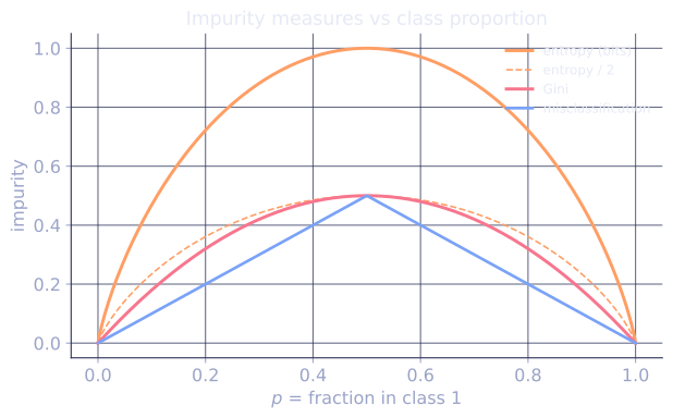
It is the probability of misclassification under a stochastic decision rule that predicts class $k$ with probability $p_k$. Gini is 0 when one class dominates ($p_k = 1$ for one $k$) and maximized at the uniform distribution ($\text{Gini} = 1 - 1/K$).

Entropy and information gain

For the same proportions,

This is the Shannon entropy in bits. It equals 0 for pure nodes and $\log_2 K$ at the uniform distribution. The information gain of a split is the expected reduction in entropy:

Trees built with information gain are called ID3 / C4.5 trees in the classical literature.

Gini and entropy track each other closely; the binary case $\text{Gini} = 2p(1 - p)$ and $H = -p\log_2 p - (1-p)\log_2(1-p)$ both peak at $p = 0.5$. They differ in computational cost (Gini is cheaper, no logarithm) and in marginal sensitivity to small probabilities (entropy is more sensitive). In practice the trees they produce are nearly indistinguishable.

MSE for regression

For a node with target values $y_1, \dots, y_n$, the mean squared error impurity is the variance:

The optimal leaf prediction is the mean $\bar y$ (which is exactly OLS for a constant predictor). A split reduces MSE by partitioning the data into two groups whose individual variances sum to less than the parent variance.

Mean absolute error (MAE) can replace MSE for more robust regression trees, but the closed-form best leaf becomes the median rather than the mean.

Why information-gain-style criteria favor balanced splits

A split is more useful when its two children are both reasonably large. A split that isolates a single point gives high purity in that child but very small $|S_L|$ in the weighted sum, so the gain is dominated by the other child. Gain criteria automatically discount tiny-child splits, mitigating one common failure mode.

Overfitting and noise

Without limits, recursive splitting drives every leaf to perfect purity by isolating noise. Even a single mislabeled point can drive several extra splits. The remedies are the subject of the next lesson:

• Max depth (cap recursion).
• Min samples per leaf (refuse small leaves).
• Min impurity decrease (refuse splits that barely help).
• Cost-complexity pruning (remove subtrees that don't justify their size).

The right amount of regularization is found by cross-validation.

Check it on arrays

import numpy as np

rng = np.random.default_rng(0)

def gini(labels):
    p = np.bincount(labels) / len(labels)
    return 1 - np.sum(p**2)

def entropy(labels):
    p = np.bincount(labels) / len(labels)
    nz = p[p > 0]
    return -np.sum(nz * np.log2(nz))

# Both impurities peak at the uniform distribution and vanish at purity
for p in [0.0, 0.1, 0.5, 0.9, 1.0]:
    n = 1000
    y = (rng.random(n) < p).astype(int)
    print(f"p={p}: gini={gini(y):.3f}, entropy={entropy(y):.3f} bits")

# Information gain of a useful split vs a useless one
y_parent = np.concatenate([np.zeros(100), np.ones(100)]).astype(int)
y_left_good = np.zeros(100, dtype=int)
y_right_good = np.ones(100, dtype=int)
y_left_bad = np.concatenate([np.zeros(50), np.ones(50)]).astype(int)
y_right_bad = np.concatenate([np.zeros(50), np.ones(50)]).astype(int)

ig_good = entropy(y_parent) - 0.5 * entropy(y_left_good) - 0.5 * entropy(y_right_good)
ig_bad = entropy(y_parent) - 0.5 * entropy(y_left_bad) - 0.5 * entropy(y_right_bad)
print(f"\nperfect split IG = {ig_good:.3f} bits  (= H(parent), one full bit recovered)")
print(f"useless split IG = {ig_bad:.3f} bits  (no information)")

# MSE impurity for regression
y_reg_parent = rng.normal(size=200)
y_reg_left = y_reg_parent[y_reg_parent < 0]
y_reg_right = y_reg_parent[y_reg_parent >= 0]
parent_var = np.var(y_reg_parent)
weighted_child = (len(y_reg_left) * np.var(y_reg_left) + len(y_reg_right) * np.var(y_reg_right)) / len(y_reg_parent)
print(f"\nregression MSE parent: {parent_var:.3f}, after split: {weighted_child:.3f}, reduction: {parent_var - weighted_child:.3f}")

The two classification criteria behave as advertised; the perfect split recovers a full bit of information while the uninformative one yields zero; and the regression split halves the variance on a symmetric distribution.

Exercises

Exercise 1. A node holds 80 examples: 60 of class A and 20 of class B. A split sends 40 examples (30 A, 10 B) left and 40 examples (30 A, 10 B) right. Compute the parent Gini, both child Ginis, and the Gini gain. Explain the result.

Exercise 2. Show that for a binary node with class proportions $p$ and $1 - p$, the Gini impurity equals $2p(1 - p)$. Then verify it peaks at $p = 0.5$ by setting the derivative to zero.

Exercise 3 (code). The lesson claims a split that isolates a single point gives high child purity but little gain, because its weight in the sum is tiny. Verify this: on a 200-point node with a 50/50 class mix, compare the Gini gain of a balanced perfect split against a split that peels off one point.

import numpy as np

def gini(labels):
    if len(labels) == 0: return 0.0
    p = np.bincount(labels, minlength=2) / len(labels)
    return 1 - np.sum(p**2)

def gain(y, mask):
    n = len(y)
    return gini(y) - (mask.sum()/n)*gini(y[mask]) - ((~mask).sum()/n)*gini(y[~mask])

y = np.concatenate([np.zeros(100), np.ones(100)]).astype(int)

balanced = np.arange(200) < 100              # left = all class 0, right = all class 1
peel_one = np.arange(200) < 1                # left = one class-0 point only

g_balanced = gain(y, balanced)
g_peel = gain(y, peel_one)

assert np.isclose(g_balanced, 0.5)           # perfect split recovers full Gini 0.5
assert g_peel < 0.01                         # isolating one point barely helps
print(f"balanced perfect split gain: {g_balanced:.4f}")
print(f"peel-one-point gain:         {g_peel:.4f}")

The next lesson controls the resulting tree size so it generalizes instead of memorizing.

References

- [1]Breiman, L., Friedman, J., Olshen, R., & Stone, C. (1984). Classification and Regression Trees. Wadsworth. Gini impurity for classification and squared-error impurity for regression.↩
- [2]Hastie, T., Tibshirani, R., & Friedman, J. (2009). The Elements of Statistical Learning (2nd ed.). Springer. Impurity measures and information gain (doi:10.1007/978-0-387-84858-7).↩