Tree feature importance

Compare Gini-impurity importance against permutation importance and know when each lies.

⏱ 24 minPrerequisites:Bagging and random forests

Tree ensembles are not black boxes: their structure exposes which features the model relies on. Two standard measures: Gini importance (built from internal splits) and permutation importance (model-agnostic)[1]. Both are useful; each has a characteristic way of misleading[2].

Gini (mean decrease in impurity)

For a fitted tree, the importance of feature $j$ is the total impurity reduction summed across all splits on $j$ , weighted by the fraction of samples reaching each split:

\text{imp}(j) = \sum_{\text{nodes splitting on } j} \frac{|S_{\text{node}}|}{n}\,\Delta_{\text{node}}.

For an ensemble, average across trees. The result is the mean decrease in impurity (MDI) importance, available essentially for free during training.

Failure mode: MDI is biased toward features with many distinct values (high cardinality categoricals, continuous features). The bias comes from having more candidate thresholds to find a spurious gain in. On synthetic data with truly irrelevant high-cardinality features, MDI will rank them above the relevant ones.

Permutation importance

Train the model, measure baseline performance on a held-out set. For each feature $j$ , permute its values across the test set (breaking the feature-target relationship), measure performance again, and report the drop:

\text{perm}(j) = \text{score}_{\text{baseline}} - \text{score}_{\text{permuted } j}.

A feature the model genuinely relies on shows a large drop. A feature the model ignores shows ~zero drop, even if it had high cardinality.

Failure mode: with correlated features, permuting one feature leaves the model still able to read the same signal through the correlated partner, underestimating both features' importance. Standard remedy: group correlated features and permute them together.

When to use which

Quick interpretability during training: MDI is free and usually correct enough on real data without pathological high-cardinality features.
Defensible feature ranking for downstream decisions: permutation importance on a held-out set, with grouped permutations when correlation is high.
Causal questions: neither. Feature importance reports what the model uses, not what the world causes. For causal questions, do an intervention or use causal-inference methods (pillar B).

Beyond global importance

Both methods give one number per feature averaged over the dataset. For per-prediction explanations:

Tree SHAP: an efficient algorithm for SHAP values on tree ensembles, decomposing each prediction into feature contributions exactly.
Partial dependence plots: trace the model's average prediction as one feature varies, marginalizing over the rest.
Individual conditional expectation (ICE): same as partial dependence but per-sample, revealing heterogeneous effects.

Impurity (MDI) importance inflates a feature that merely copies a real signal, whereas permutation importance discounts the redundant copy.

Check it on arrays

python · numpy

import numpy as np

rng = np.random.default_rng(0)

# Synthetic data: features 0,1 truly drive y; features 2,3 are irrelevant.
# Feature 4 is correlated with feature 0 (the MDI / permutation pitfall).
n, d = 500, 5
X = rng.normal(size=(n, d))
X[:, 4] = X[:, 0] + 0.1 * rng.normal(size=n)            # correlated with feature 0
y = ((X[:, 0] + X[:, 1] > 0)).astype(int)

def gini(labels):
    if len(labels) == 0: return 0.0
    p = np.bincount(labels, minlength=2) / len(labels)
    return 1 - np.sum(p**2)

class Node:
    def __init__(self): self.leaf = self.feature = self.threshold = self.left = self.right = None
    feature = threshold = left = right = leaf = None

def split(X, y):
    n, d = X.shape; best = (None, None, -1); parent = gini(y)
    for j in range(d):
        for t in np.unique(X[:, j]):
            m = X[:, j] <= t
            if m.sum() == 0 or (~m).sum() == 0: continue
            gain = parent - (m.sum()/n)*gini(y[m]) - ((~m).sum()/n)*gini(y[~m])
            if gain > best[2]: best = (j, t, gain)
    return best

def build(X, y, max_depth=6, importance=None, total_n=None):
    if importance is None: importance = np.zeros(X.shape[1])
    if total_n is None: total_n = len(y)
    node = Node()
    if max_depth == 0 or len(y) < 2 or gini(y) == 0:
        node.leaf = int(np.argmax(np.bincount(y, minlength=2))); return node, importance
    j, t, gain = split(X, y)
    if j is None or gain <= 0:
        node.leaf = int(np.argmax(np.bincount(y, minlength=2))); return node, importance
    importance[j] += (len(y) / total_n) * gain
    m = X[:, j] <= t; node.feature, node.threshold = j, t
    node.left, importance = build(X[m], y[m], max_depth - 1, importance, total_n)
    node.right, importance = build(X[~m], y[~m], max_depth - 1, importance, total_n)
    return node, importance

def predict(node, x):
    while node.leaf is None:
        node = node.left if x[node.feature] <= node.threshold else node.right
    return node.leaf

# Fit one tree, report MDI
tree, mdi = build(X, y)
mdi /= mdi.sum()
print("MDI importance:        ", np.round(mdi, 3))

# Permutation importance on a held-out set
idx = rng.permutation(n); tr, te = idx[:300], idx[300:]
tree, _ = build(X[tr], y[tr])
y_pred = np.array([predict(tree, x) for x in X[te]])
baseline = np.mean(y_pred == y[te])

perm = np.zeros(d)
for j in range(d):
    X_te_p = X[te].copy()
    rng.shuffle(X_te_p[:, j])
    y_pred_p = np.array([predict(tree, x) for x in X_te_p])
    perm[j] = baseline - np.mean(y_pred_p == y[te])

print(f"baseline test acc:     {baseline:.3f}")
print("permutation importance:", np.round(perm, 3))
print("\nNote: feature 0 + feature 4 are correlated; permutation importance")
print("splits the credit and underestimates each individually.")

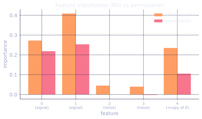
MDI ranks the truly informative features 0 and 1 highest; permutation importance confirms but underrates the correlated pair.

Exercises

Exercise 1. A single split on feature $j$ sits at a node holding 100 of the forest's 400 training examples and reduces Gini by $\Delta = 0.2$ . It is the only split on $j$ in the tree. Compute its MDI contribution using the weighted-gain formula, and state how the contribution changes if the same split instead sat at a node holding only 20 examples.

Solution

Step 1. The MDI contribution of a split is $\frac{|S_{\text{node}}|}{n}\, \Delta_{\text{node}}$ . With $|S_{\text{node}}| = 100$ , $n = 400$ , $\Delta = 0.2$ :

\frac{100}{400}\cdot 0.2 = 0.25 \cdot 0.2 = 0.05.

Step 2. At a node holding 20 examples with the same $\Delta = 0.2$ :

\frac{20}{400}\cdot 0.2 = 0.05 \cdot 0.2 = 0.01.

Step 3. The same impurity drop contributes five times less when it happens deeper in the tree on fewer samples. MDI weights each split by the fraction of data reaching it, so high splits near the root dominate a feature's importance.

Exercise 2. The lesson says permutation importance splits the credit between two correlated features and underestimates each. Explain mechanically why, and predict what grouped permutation (shuffling both together) reports instead.

Solution

Step 1. Permutation importance of feature $j$ is the accuracy drop when only $j$ is shuffled. If feature $k$ is highly correlated with $j$ , the model can read nearly the same signal through $k$ after $j$ is destroyed.

Step 2. So shuffling $j$ alone barely hurts accuracy (the partner $k$ carries the signal), and shuffling $k$ alone barely hurts either. Each individual importance is small, even though the underlying signal is strong: the credit is split, and both look weak.

Step 3. Shuffling $j$ and $k$ together destroys the shared signal with no surviving partner, so accuracy drops by the full amount the signal was worth. The grouped permutation recovers the true combined importance that the two single-feature permutations each undercounted.

Exercise 3 (code). Build a dataset with a truly relevant low-cardinality feature and a truly irrelevant high-cardinality feature (many distinct values). Fit a tree, compute MDI, and confirm the cardinality bias: the irrelevant high-cardinality feature receives nonzero MDI it does not deserve.

Solution

Step 1. Make feature 0 a clean binary predictor of $y$ and feature 1 pure noise with a distinct value per row (maximum cardinality). Fit the lesson's importance-accumulating tree and read off MDI.

python · numpy

import numpy as np

rng = np.random.default_rng(0)
n = 400
X = np.zeros((n, 2))
X[:, 0] = (rng.random(n) < 0.5).astype(float)      # low-cardinality, relevant
X[:, 1] = rng.random(n)                              # high-cardinality, irrelevant
y = X[:, 0].astype(int)                              # y depends only on feature 0
y[rng.random(n) < 0.1] ^= 1                          # 10% label noise

def gini(labels):
    if len(labels) == 0: return 0.0
    p = np.bincount(labels, minlength=2) / len(labels)
    return 1 - np.sum(p**2)

class Node:
    def __init__(self): self.leaf = self.feature = self.threshold = self.left = self.right = None

def split(X, y):
    n, d = X.shape; best = (None, None, -1); parent = gini(y)
    for j in range(d):
        for t in np.unique(X[:, j]):
            m = X[:, j] <= t
            if m.sum() == 0 or (~m).sum() == 0: continue
            gain = parent - (m.sum()/n)*gini(y[m]) - ((~m).sum()/n)*gini(y[~m])
            if gain > best[2]: best = (j, t, gain)
    return best

def build(X, y, max_depth, imp, total_n):
    node = Node()
    if max_depth == 0 or len(y) < 2 or gini(y) == 0:
        node.leaf = int(np.argmax(np.bincount(y, minlength=2))); return node
    j, t, gain = split(X, y)
    if j is None or gain <= 0:
        node.leaf = int(np.argmax(np.bincount(y, minlength=2))); return node
    imp[j] += (len(y) / total_n) * gain
    m = X[:, j] <= t; node.feature, node.threshold = j, t
    node.left = build(X[m], y[m], max_depth - 1, imp, total_n)
    node.right = build(X[~m], y[~m], max_depth - 1, imp, total_n)
    return node

imp = np.zeros(2)
build(X, y, max_depth=8, imp=imp, total_n=n)
mdi = imp / imp.sum()

assert mdi[0] > mdi[1]                               # relevant feature still ranks first
assert mdi[1] > 0                                    # but the noise feature steals some credit
print(f"MDI: relevant {mdi[0]:.3f}, irrelevant-high-cardinality {mdi[1]:.3f}")

Step 2. Feature 0 keeps the larger share, but the irrelevant continuous feature 1 collects nonzero MDI. Its many candidate thresholds let deeper splits find spurious gains on the noise, the cardinality bias the lesson warns about. Permutation importance on a held-out set would discount feature 1 toward zero.

This closes the single-tree thread; the next lesson moves to boosting, where trees are added sequentially to fix each other's mistakes.

References

[1]Breiman, L. (2001). "Random forests". Machine Learning, 45(1), 5-32. Permutation importance and mean decrease in impurity for forests (doi:10.1023/A:1010933404324).↩
[2]Hastie, T., Tibshirani, R., & Friedman, J. (2009). The Elements of Statistical Learning (2nd ed.). Springer. Variable importance and its cardinality bias (doi:10.1007/978-0-387-84858-7).↩