AdaBoost

Bagging averages many trees fit to perturbed copies of the data, reducing variance. Boosting takes the opposite approach: fit weak learners sequentially, each one trained to correct the previous ensemble's mistakes. AdaBoost (adaptive boosting) is the original[1], and its analysis as exponential-loss minimization seeds the modern gradient-boosting view[2].

The algorithm

For binary labels $y_i \in \{-1, +1\}$:

1. Initialize weights $w_i^{(1)} = 1/n$.
2. For $t = 1, \dots, T$:
   • Fit a weak learner $h_t: \mathcal{X} \to \{-1, +1\}$ minimizing the weighted error $\varepsilon_t = \sum_i w_i^{(t)}\,\mathbf{1}[h_t(x_i) \ne y_i]$.
   • Compute its weight in the ensemble: $\alpha_t = \tfrac{1}{2}\log\!\frac{1 - \varepsilon_t}{\varepsilon_t}.$
   • Update example weights: $w_i^{(t+1)} \propto w_i^{(t)} \exp(-\alpha_t\, y_i\, h_t(x_i)).$
3. Return the additive predictor $H(x) = \operatorname{sign}\!\left(\sum_t \alpha_t h_t(x)\right)$.

Each round upweights misclassified points (the exponent is positive when $y_i\, h_t(x_i) = -1$), pulling the next learner's attention toward them. Correctly classified points are downweighted.

Weak learners

A weak learner does only marginally better than random guessing ($\varepsilon < 1/2$). For tabular problems the usual choice is a decision stump (a one-split tree). Stumps are deliberately underpowered, so each one captures a tiny piece of structure, and boosting builds the full classifier from their sum.

When $\varepsilon_t = 1/2$ exactly, $\alpha_t = 0$ and the round contributes nothing. When $\varepsilon_t \to 0$, $\alpha_t \to \infty$: a perfect weak learner gets full weight.

AdaBoost as exponential-loss minimization

The remarkable connection: AdaBoost is stagewise additive modeling with the exponential loss $\ell(y, F) = \exp(-y F)$.

Theorem. Define $F_T(x) = \sum_{t=1}^T \alpha_t h_t(x)$. AdaBoost's choice of $(h_t, \alpha_t)$ at round $t$ is exactly the pair that minimizes

over all $(h, \alpha)$, with $F_{t-1}$ fixed.

Sketch. Set $w_i^{(t)} = \exp(-y_i F_{t-1}(x_i))/Z_t$. The objective factors as $\sum_i w_i^{(t)}\exp(-y_i \alpha h(x_i))$. For a $\pm 1$-valued $h$, split the sum into correctly and incorrectly classified groups; the inner minimization in $\alpha$ for fixed $h$ gives the AdaBoost formula for $\alpha_t$ and the outer one in $h$ becomes the weighted-error minimization.

This recasting matters because it generalizes: swap the exponential loss for any differentiable loss and the algorithm becomes gradient boosting (next lesson).

Why AdaBoost works

• Bias reduction: each weak learner is high-bias, but the sum can fit arbitrarily complex functions. The training error decays exponentially in $T$ for weak learners with edge.
• Margin maximization: even after training error hits zero, more rounds keep increasing the margin $y_i F(x_i)/\sum_t |\alpha_t|$, which generally improves test performance. This is why AdaBoost often does not overfit even with many rounds.

Failure modes

• Label noise wrecks AdaBoost. Mislabeled points get exponentially upweighted, and the ensemble chases them. Regularized variants (LogitBoost, GentleBoost) help.
• Computational: each round refits on reweighted data, and the rounds are sequential. Random forests can train each tree in parallel; boosting cannot.

Check it on arrays

import numpy as np

rng = np.random.default_rng(0)

n, d = 400, 2
X = rng.normal(size=(n, d))
y = np.sign(X[:, 0] * X[:, 1] - 0.3 + 0.4 * rng.normal(size=n))

def weighted_stump(X, y, w):
    """Best 1-split stump: feature, threshold, sign, weighted error."""
    n, d = X.shape
    best = (None, None, 1, 1.0)
    for j in range(d):
        order = np.argsort(X[:, j])
        for k in range(1, n):
            t = (X[order[k - 1], j] + X[order[k], j]) / 2
            for sign in (+1, -1):
                pred = sign * np.where(X[:, j] <= t, +1, -1)
                err = np.sum(w * (pred != y))
                if err < best[3]:
                    best = (j, t, sign, err)
    return best

def adaboost(X, y, T=30):
    n = len(y)
    w = np.full(n, 1 / n)
    stumps, alphas = [], []
    for _ in range(T):
        j, t, sign, eps = weighted_stump(X, y, w)
        if eps >= 0.5 - 1e-9: break
        alpha = 0.5 * np.log((1 - eps) / max(eps, 1e-12))
        pred = sign * np.where(X[:, j] <= t, +1, -1)
        w = w * np.exp(-alpha * y * pred); w /= w.sum()
        stumps.append((j, t, sign)); alphas.append(alpha)
    return stumps, alphas

def ada_predict(X, stumps, alphas):
    F = np.zeros(len(X))
    for (j, t, sign), a in zip(stumps, alphas):
        F += a * sign * np.where(X[:, j] <= t, +1, -1)
    return np.sign(F)

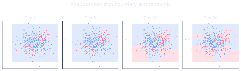
# Try increasing T and watch train + held-out
idx = rng.permutation(n); tr, te = idx[:300], idx[300:]
for T in [1, 5, 20, 50]:
    stumps, alphas = adaboost(X[tr], y[tr], T=T)
    tr_acc = np.mean(ada_predict(X[tr], stumps, alphas) == y[tr])
    te_acc = np.mean(ada_predict(X[te], stumps, alphas) == y[te])
    print(f"T={T:>2}: train acc={tr_acc:.3f}  test acc={te_acc:.3f}  (stumps used: {len(stumps)})")

Training accuracy climbs as more stumps are added; test accuracy also improves and then plateaus.

Exercises

Exercise 1. A weak learner at round $t$ achieves weighted error $\varepsilon_t = 0.25$. Compute its ensemble weight $\alpha_t$, and the unnormalized weight-update multiplier $\exp(-\alpha_t y_i h_t(x_i))$ for a correctly classified example and for a misclassified one.

Exercise 2. Show that after the round-$t$ update with the AdaBoost choice of $\alpha_t$, the reweighted distribution makes the current weak learner $h_t$ look like random guessing: its weighted error under $w^{(t+1)}$ equals $1/2$.

Exercise 3 (code). Run one AdaBoost round by hand in numpy. Given fixed stump predictions and labels, compute the weighted error, $\alpha_t$, and the updated normalized weights, then verify the property from Exercise 2: the stump's weighted error under the new weights is $1/2$.

import numpy as np

y    = np.array([+1, +1, -1, -1, +1, -1, +1, -1], dtype=float)
pred = np.array([+1, -1, -1, -1, +1, +1, +1, -1], dtype=float)   # 2 of 8 wrong

w = np.full(len(y), 1 / len(y))
eps = np.sum(w * (pred != y))
alpha = 0.5 * np.log((1 - eps) / eps)

w_new = w * np.exp(-alpha * y * pred)
w_new /= w_new.sum()

eps_new = np.sum(w_new * (pred != y))

assert np.isclose(eps, 0.25)              # 2 wrong out of 8 under uniform weights
assert np.isclose(eps_new, 0.5)           # reweighting neutralizes this stump
print(f"eps={eps:.3f}, alpha={alpha:.3f}, eps under new weights={eps_new:.3f}")

The next lesson generalizes this idea to any differentiable loss with gradient boosting.

References

- [1]Freund, Y., & Schapire, R. E. (1997). "A decision-theoretic generalization of on-line learning and an application to boosting". Journal of Computer and System Sciences, 55(1), 119-139. The original AdaBoost algorithm (doi:10.1006/jcss.1997.1504).↩
- [2]Hastie, T., Tibshirani, R., & Friedman, J. (2009). The Elements of Statistical Learning (2nd ed.). Springer. AdaBoost as stagewise additive modeling with exponential loss (doi:10.1007/978-0-387-84858-7).↩