Bagging and random forests

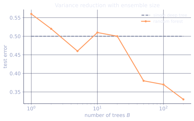
Trees are high-variance learners: small data changes produce very different trees. Bagging (bootstrap aggregating) averages many trees fit on bootstrap resamples of the data, slashing the variance without adding bias[1]. Random forests push the idea further by also randomizing which features each split can use, which decorrelates the trees and lowers variance even more[2].

Variance reduction from averaging

Let $\hat f_b(x)$ be the prediction of the $b$-th tree, trained on a different bootstrap sample of the data. The bagged predictor averages them:

If the individual predictors are i.i.d. with variance $\sigma^2$, the average has variance $\sigma^2 / B$. The catch: bootstrap-trained trees are not independent (they share most of the same training data), so the variance of the average is

where $\rho$ is the average correlation between trees. As $B \to \infty$, the variance floors at $\rho\sigma^2$. Reducing $\rho$ is what random forests add on top of bagging[3].

The random-forest twist

At each split, instead of picking the best feature among all $d$ features, pick the best among a random subset of $m$ features. Typical choices: $m = \sqrt d$ for classification, $m = d/3$ for regression. The randomness ensures that no single dominant feature appears in every tree, so trees see different subsets of structure and end up less correlated.

The cost is per-tree quality: a tree restricted to subset $m$ usually beats its larger-$m$ counterpart in training loss. The forest still wins because the ensemble variance reduction more than compensates.

Out-of-bag (OOB) estimation

A bootstrap sample contains roughly 63% unique training examples (since $1 - (1 - 1/n)^n \to 1 - 1/e \approx 0.632$). The remaining 37% are out-of-bag for that tree. Predicting an OOB example with only the trees that did not see it gives a free held-out estimate of test error, without a separate validation set.

For a random forest, the OOB error tracks held-out test error closely. It is the practical replacement for cross-validation on small datasets.

Hyperparameters

The standard knobs:

• Number of trees $B$. Effectively a noise control: more trees never hurt accuracy and modestly help calibration; pick $B$ as large as compute allows.
• max_features $m$. Smaller $m$ means lower correlation and lower variance, but each tree fits worse.
• max_depth / min_samples_leaf. Less critical than in single trees, but useful for compute control.

Defaults usually work; the most useful tunable is $m$.

Strengths and limits

Strengths:

• Excellent out-of-the-box accuracy on tabular data.
• OOB error replaces cross-validation.
• Handles mixed types and missing values gracefully.
• Robust to irrelevant features and outliers.

Limits:

• Less accurate than gradient boosting on most tabular benchmarks.
• Predictions are bounded by the training-target range (extrapolation is weak).
• Many trees means slower inference and bigger model files.

Check it on arrays

import numpy as np

rng = np.random.default_rng(0)

n, d = 400, 6
X = rng.normal(size=(n, d))
y = ((X[:, 0] + X[:, 1] > 0) ^ (X[:, 2] > 0)).astype(int)
flip = rng.random(n) < 0.10
y = np.where(flip, 1 - y, y)

def gini(labels):
    if len(labels) == 0: return 0.0
    p = np.bincount(labels, minlength=2) / len(labels)
    return 1 - np.sum(p**2)

class Node:
    def __init__(self): self.leaf = None; self.feature = self.threshold = self.left = self.right = None

def split(X, y, m, rng):
    n, d = X.shape
    feats = rng.choice(d, size=min(m, d), replace=False)
    best = (None, None, -1)
    parent = gini(y)
    for j in feats:
        for t in np.unique(X[:, j]):
            mm = X[:, j] <= t
            if mm.sum() == 0 or (~mm).sum() == 0: continue
            gain = parent - (mm.sum()/n)*gini(y[mm]) - ((~mm).sum()/n)*gini(y[~mm])
            if gain > best[2]: best = (j, t, gain)
    return best

def build(X, y, m, rng, max_depth=8):
    node = Node()
    if max_depth == 0 or len(y) < 2 or gini(y) == 0:
        node.leaf = int(np.argmax(np.bincount(y, minlength=2))); return node
    j, t, gain = split(X, y, m, rng)
    if j is None or gain <= 0:
        node.leaf = int(np.argmax(np.bincount(y, minlength=2))); return node
    mm = X[:, j] <= t
    node.feature, node.threshold = j, t
    node.left = build(X[mm], y[mm], m, rng, max_depth - 1)
    node.right = build(X[~mm], y[~mm], m, rng, max_depth - 1)
    return node

def predict(node, x):
    while node.leaf is None:
        node = node.left if x[node.feature] <= node.threshold else node.right
    return node.leaf

# Random forest
idx_te = rng.choice(n, size=100, replace=False)
idx_tr = np.setdiff1d(np.arange(n), idx_te)
Xtr, ytr = X[idx_tr], y[idx_tr]
Xte, yte = X[idx_te], y[idx_te]

def random_forest(Xtr, ytr, B=50, m=2, rng=rng):
    trees, oob_idx = [], []
    n_tr = len(ytr)
    for _ in range(B):
        sample = rng.integers(0, n_tr, n_tr)
        trees.append(build(Xtr[sample], ytr[sample], m=m, rng=rng))
        oob_idx.append(np.setdiff1d(np.arange(n_tr), sample))
    return trees, oob_idx

trees, oob_idx = random_forest(Xtr, ytr, B=50, m=2, rng=rng)
pred_te = np.mean([[predict(t, x) for x in Xte] for t in trees], axis=0)
acc_te = np.mean((pred_te > 0.5) == yte)
print(f"random-forest test acc: {acc_te:.3f}")

# OOB error: for each training point, average predictions from trees that did not see it
counts = np.zeros(len(ytr))
votes = np.zeros(len(ytr))
for tree, oob in zip(trees, oob_idx):
    for i in oob:
        votes[i] += predict(tree, Xtr[i]); counts[i] += 1
mask = counts > 0
oob_pred = votes[mask] / counts[mask]
oob_acc = np.mean((oob_pred > 0.5) == ytr[mask])
print(f"OOB accuracy:        {oob_acc:.3f}  "
      f"(over {int(mask.sum())}/{len(ytr)} examples with >=1 OOB tree)")

# Single tree vs forest
single = build(Xtr, ytr, m=d, rng=rng, max_depth=8)
single_acc = np.mean([predict(single, x) for x in Xte] == yte)
print(f"single tree test acc: {single_acc:.3f}  (forest reduces variance over this)")

The random forest beats the single tree on the noisy test set, and the OOB accuracy tracks the held-out test accuracy.

Exercises

Exercise 1. Using the variance bound $\rho\sigma^2 + \frac{1-\rho}{B}\sigma^2$ for the average of $B$ trees, take $\sigma^2 = 1$. Compute the limiting variance as $B \to \infty$ for $\rho = 0.6$ (plain bagged trees) and $\rho = 0.1$ (decorrelated forest trees), and the variance at $B = 50$ for each. Explain what the two numbers say about why random forests help.

Exercise 2. The lesson states a bootstrap sample of size $n$ contains about 63% unique examples. Derive the $1 - 1/e$ limit, and explain why the remaining fraction is the out-of-bag set used for free error estimation.

Exercise 3 (code). Demonstrate decorrelation directly: fit two ensembles on the same data, one choosing the best split among all features ($m = d$, plain bagging) and one among a random subset ($m = 2$). Estimate the average pairwise correlation of tree predictions in each, and confirm the random-subset forest is less correlated.

import numpy as np

rng = np.random.default_rng(0)
n, d = 400, 6
X = rng.normal(size=(n, d))
y = ((X[:, 0] + X[:, 1] > 0) ^ (X[:, 2] > 0)).astype(int)

def gini(labels):
    if len(labels) == 0: return 0.0
    p = np.bincount(labels, minlength=2) / len(labels)
    return 1 - np.sum(p**2)

class Node:
    def __init__(self): self.leaf = self.feature = self.threshold = self.left = self.right = None

def split(X, y, m, rng):
    n, d = X.shape
    feats = rng.choice(d, size=min(m, d), replace=False)
    best = (None, None, -1); parent = gini(y)
    for j in feats:
        for t in np.unique(X[:, j]):
            mm = X[:, j] <= t
            if mm.sum() == 0 or (~mm).sum() == 0: continue
            gain = parent - (mm.sum()/n)*gini(y[mm]) - ((~mm).sum()/n)*gini(y[~mm])
            if gain > best[2]: best = (j, t, gain)
    return best

def build(X, y, m, rng, max_depth=6):
    node = Node()
    if max_depth == 0 or len(y) < 2 or gini(y) == 0:
        node.leaf = int(np.argmax(np.bincount(y, minlength=2))); return node
    j, t, gain = split(X, y, m, rng)
    if j is None or gain <= 0:
        node.leaf = int(np.argmax(np.bincount(y, minlength=2))); return node
    mm = X[:, j] <= t; node.feature, node.threshold = j, t
    node.left = build(X[mm], y[mm], m, rng, max_depth - 1)
    node.right = build(X[~mm], y[~mm], m, rng, max_depth - 1)
    return node

def predict(node, x):
    while node.leaf is None:
        node = node.left if x[node.feature] <= node.threshold else node.right
    return node.leaf

Xtr, ytr, Xte = X[:300], y[:300], X[300:]

def mean_pairwise_corr(m, B=25):
    preds = []
    for _ in range(B):
        s = rng.integers(0, len(ytr), len(ytr))
        tree = build(Xtr[s], ytr[s], m=m, rng=rng)
        preds.append([predict(tree, x) for x in Xte])
    P = np.array(preds, float)
    P = P[P.std(axis=1) > 0]                 # drop constant-prediction trees
    C = np.corrcoef(P)
    off = C[np.triu_indices_from(C, k=1)]
    return np.nanmean(off)

corr_full = mean_pairwise_corr(m=6)          # plain bagging, all features
corr_sub = mean_pairwise_corr(m=2)           # random subset
assert corr_sub < corr_full                  # random subsets decorrelate trees
print(f"mean tree correlation: m=d {corr_full:.3f}, m=2 {corr_sub:.3f}")

The next lesson opens the black box: how to read feature importance from a forest.

References

- [1]Breiman, L. (1996). "Bagging predictors". Machine Learning, 24(2), 123-140. Bootstrap aggregation as a variance-reduction scheme (doi:10.1007/BF00058655).↩
- [2]Breiman, L. (2001). "Random forests". Machine Learning, 45(1), 5-32. Decorrelating bagged trees with random feature subsets (doi:10.1023/A:1010933404324).↩
- [3]Hastie, T., Tibshirani, R., & Friedman, J. (2009). The Elements of Statistical Learning (2nd ed.). Springer. The correlation-variance bound for averaged predictors (doi:10.1007/978-0-387-84858-7).↩