Decision trees

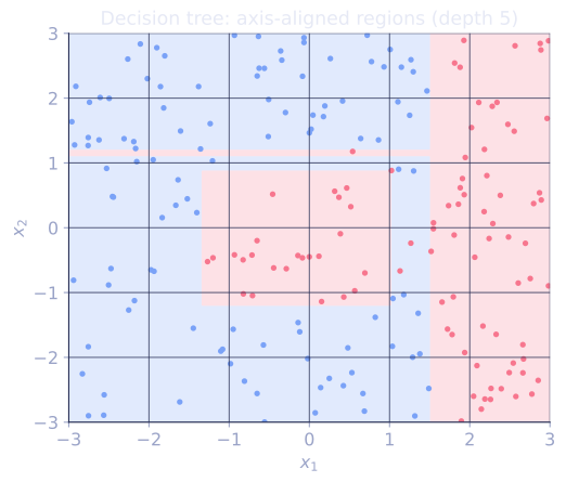
A decision tree partitions the input space with a sequence of axis-aligned splits and predicts a constant in each region[1]. The recursive structure makes trees natural to read, fast to evaluate, and easy to extend; they are also the building block of the most successful tabular learners (random forests, gradient boosting)[2].

The structure

A binary decision tree has internal nodes that test one feature against a threshold and leaves that emit a prediction:

• Internal node: "is $x_j \le t$?" Each test routes the input to a left or right child.
• Leaf: a constant prediction (a class label for classification, a real number for regression).

A path from root to leaf is a conjunction of tests, and the leaf is the predicted output for any input matching all the tests on the path. Together the leaves partition the input space into axis-aligned rectangles, and the tree's prediction is piecewise constant.

Recursive partitioning

Greedy training: at each node, pick the split that most improves the chosen quality measure on the data currently at the node, then recurse on the two children. Stop when a node is pure (all labels equal), small (fewer than $n_{\min}$ examples), or deep (beyond a max depth).

For a node containing data subset $S$:

1. For every feature $j$ and candidate threshold $t$, compute the impurity of the children after splitting on $(j, t)$.
2. Pick the split that maximizes the impurity reduction $\Delta = \text{Imp}(S) - \frac{|S_L|}{|S|}\text{Imp}(S_L) - \frac{|S_R|}{|S|}\text{Imp}(S_R)$.
3. Recurse on $S_L$ and $S_R$.

Candidate thresholds are typically midpoints between consecutive sorted feature values, so the search is $O(n \log n)$ per feature.

Prediction

For classification, each leaf stores the majority class (or class probabilities estimated as label frequencies). For regression, each leaf stores the mean of its training targets. Evaluation walks one root-to-leaf path, costing $O(\text{depth})$.

Strengths and weaknesses

Strengths:

• Interpretable: each leaf has a readable conjunction of rules.
• Handles mixed feature types natively (no scaling, no one-hot needed for the splits themselves).
• Captures interactions automatically: any conjunction of feature tests is one path.
• Fast at inference.

Weaknesses:

• High variance: a single tree changes drastically with small data perturbations. Different random subsamples produce very different trees.
• Axis-aligned splits are bad at capturing rotated or curved boundaries.
• Greedy training is locally optimal: the best first split may not lead to the globally best tree.

The high-variance failure mode motivates random forests (averaging many decorrelated trees) and gradient boosting (sequential additive trees) in the next lessons.

Check it on arrays

import numpy as np

rng = np.random.default_rng(0)

# Synthetic classification: two interleaved blobs
n = 200
X = rng.uniform(-3, 3, size=(n, 2))
y = ((X[:, 0]**2 + X[:, 1]**2 < 2) | (X[:, 0] > 1.5)).astype(int)

class TreeNode:
    def __init__(self):
        self.feature = self.threshold = self.left = self.right = self.leaf_pred = None

def gini(labels):
    if len(labels) == 0: return 0.0
    p = np.bincount(labels) / len(labels)
    return 1 - np.sum(p**2)

def best_split(X, y):
    best_j, best_t, best_gain = None, None, -1e9
    parent_imp = gini(y)
    n = len(y)
    for j in range(X.shape[1]):
        vals = np.unique(X[:, j])
        thresholds = (vals[:-1] + vals[1:]) / 2
        for t in thresholds:
            mask = X[:, j] <= t
            if mask.sum() == 0 or (~mask).sum() == 0: continue
            gain = parent_imp - (mask.sum() / n) * gini(y[mask]) - ((~mask).sum() / n) * gini(y[~mask])
            if gain > best_gain:
                best_gain, best_j, best_t = gain, j, t
    return best_j, best_t, best_gain

def build_tree(X, y, depth=0, max_depth=4, min_samples=5):
    node = TreeNode()
    if len(y) <= min_samples or depth >= max_depth or len(set(y)) == 1:
        node.leaf_pred = int(np.argmax(np.bincount(y)))
        return node
    j, t, gain = best_split(X, y)
    if gain <= 1e-9:
        node.leaf_pred = int(np.argmax(np.bincount(y)))
        return node
    mask = X[:, j] <= t
    node.feature, node.threshold = j, t
    node.left = build_tree(X[mask], y[mask], depth + 1, max_depth, min_samples)
    node.right = build_tree(X[~mask], y[~mask], depth + 1, max_depth, min_samples)
    return node

def predict(node, x):
    while node.leaf_pred is None:
        node = node.left if x[node.feature] <= node.threshold else node.right
    return node.leaf_pred

tree = build_tree(X, y, max_depth=5)
y_pred = np.array([predict(tree, x) for x in X])
print(f"training accuracy: {np.mean(y_pred == y):.3f}")

def count_leaves(node):
    return 1 if node.leaf_pred is not None else count_leaves(node.left) + count_leaves(node.right)
print(f"leaves: {count_leaves(tree)}")

# High variance: different bootstrap samples give different trees
acc_bootstrap = []
for _ in range(5):
    idx = rng.integers(0, len(y), size=len(y))
    t2 = build_tree(X[idx], y[idx], max_depth=5)
    acc_bootstrap.append(np.mean([predict(t2, x) for x in X] == y))
print(f"single-tree accuracies on 5 bootstraps: {[round(a, 3) for a in acc_bootstrap]}")

The hand-rolled tree fits the training set, gives readable leaves, and shows the variance problem across bootstrap samples.

Exercises

Exercise 1. A node holds 10 examples: 6 of class 0 and 4 of class 1. A candidate split sends all 6 class-0 examples and 0 class-1 examples to the left child, and the remaining 4 class-1 examples to the right child. Compute the Gini impurity of the parent and of each child, and the impurity reduction $\Delta$ using the weighted-children formula from the lesson.

Exercise 2. The lesson says any conjunction of feature tests is one root-to-leaf path. Consider the target $y = 1$ exactly when $x_1 \le 0$ and $x_2 > 0$, and $y = 0$ otherwise. Sketch the shallowest axis-aligned tree that classifies this rule perfectly, and state how many leaves it has.

Exercise 3 (code). The lesson computes impurity reduction with Gini. Write a best_split that instead maximizes the reduction in misclassification rate (the fraction of a node not in its majority class), and confirm on a small dataset that it still finds a perfect split when one exists.

import numpy as np

rng = np.random.default_rng(0)
n = 200
X = rng.uniform(-3, 3, size=(n, 2))
y = (X[:, 0] <= 0).astype(int)              # x0 <= 0 is a perfect separator

def misclass(labels):
    if len(labels) == 0: return 0.0
    p = np.bincount(labels, minlength=2) / len(labels)
    return 1 - p.max()

def best_split(X, y):
    best_j, best_t, best_gain = None, None, -1.0
    parent = misclass(y); n = len(y)
    for j in range(X.shape[1]):
        vals = np.unique(X[:, j])
        for t in (vals[:-1] + vals[1:]) / 2:
            m = X[:, j] <= t
            if m.sum() == 0 or (~m).sum() == 0: continue
            gain = parent - (m.sum()/n)*misclass(y[m]) - ((~m).sum()/n)*misclass(y[~m])
            if gain > best_gain:
                best_gain, best_j, best_t = gain, j, t
    return best_j, best_t, best_gain

j, t, gain = best_split(X, y)
# Parent misclassification is min(p0, p1); the perfect split removes all of it.
parent_mis = misclass(y)
assert j == 0                               # picks feature 0
assert np.isclose(gain, parent_mis)         # recovers the full parent impurity
print(f"split on feature {j} at {t:.3f}, gain {gain:.3f} of parent {parent_mis:.3f}")

The next lesson formalizes the split criteria that drove the tree above.

References

- [1]Breiman, L., Friedman, J., Olshen, R., & Stone, C. (1984). Classification and Regression Trees. Wadsworth. The CART formulation of binary recursive partitioning.↩
- [2]Hastie, T., Tibshirani, R., & Friedman, J. (2009). The Elements of Statistical Learning (2nd ed.). Springer. Tree-based methods as the building block of modern tabular learners (doi:10.1007/978-0-387-84858-7).↩