 AI Knowledge Tree
Gradient boosting
Frame boosting as functional gradient descent in loss space and fit trees to negative gradients.
AdaBoost minimizes a specific loss (exponential) with a specific weak learner. Gradient boosting generalizes both: pick any differentiable loss, pick any weak learner, and at each round fit the learner to the negative gradient of the loss with respect to the current predictions[1]. The result is the dominant tabular learner of the last decade[2].
Functional gradient descent
Gradient descent in parameter space updates parameters by stepping along the negative gradient. Functional gradient descent treats the predictor itself as the optimization variable.
For a loss and a current additive predictor , the gradient with respect to the predictions is
The negative gradient points in the direction the prediction at should move to reduce the loss. Boosting fits a weak learner to (least-squares regression of features to negative gradients), then takes a step:
with a small learning rate (typically 0.01-0.1). Iterate.
Reading common losses
The recipe specializes the loss to fit the task:
| Task | Loss | Negative gradient (a.k.a. pseudo-residual) |
|---|---|---|
| Regression | Squared error | (the actual residual) |
| Regression | Absolute error $ | y - F |
| Binary class. | Log-loss (logistic) | |
| Binary class. | Exponential loss | recovers AdaBoost |
So gradient-boosted regression trees with squared loss simply fit each new tree to the residuals of the previous ensemble. The exponential loss recovers AdaBoost exactly. Log-loss boosting is what production binary classifiers use under names like GBT, GBM, LightGBM, XGBoost.
Weak learners: shallow trees
Each is usually a depth-4-to-8 regression tree (regardless of classification or regression task; the tree fits the pseudo-residuals). Why shallow:
- Shallow trees are weak learners, leaving plenty of structure for later rounds.
- Deep trees would overshoot, ruining the gradient-step interpretation.
- Sequential dependence means slow rounds compound; cheap weak learners keep total time manageable.
A few hundred to a few thousand shallow trees is typical.
Regularization
Three knobs to prevent overfitting:
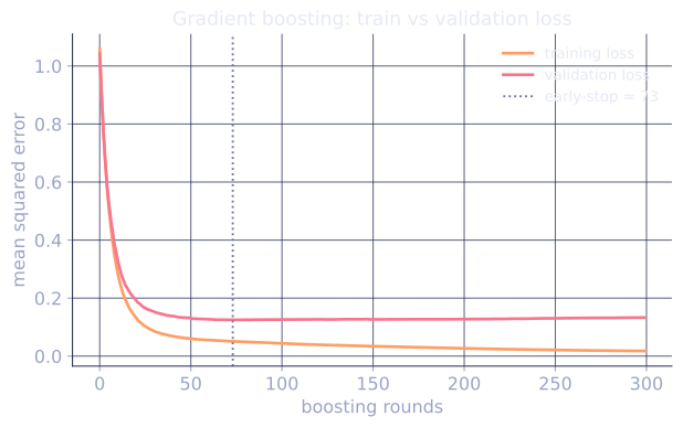
- Learning rate : smaller is safer (more rounds needed, but better generalization). The standard prescription is "fit as many trees as your budget allows with the smallest that still trains in budget".
- Subsampling: at each round, fit to a random subsample of the data (stochastic gradient boosting). Lowers variance, adds noise.
- Tree complexity: depth, min leaf size, leaf penalty. Each round's tree is the local "step", so its complexity is the step size.
Strengths
- State of the art on most tabular benchmarks, often beating deep learning by a wide margin.
- Handles mixed types, missing values, and irrelevant features.
- Predictions are bounded by training-data range, so well-behaved on interpolation.
Limits
- Sequential, not embarrassingly parallel. Each round needs the previous.
- Many hyperparameters to tune.
- Cumulative training cost can be large.
The next lesson covers the production-grade variants (XGBoost, LightGBM) that squeeze speed and accuracy out of this template.
Check it on arrays
import numpy as np

rng = np.random.default_rng(0)

# Regression target with structure + noise
n = 600
X = rng.uniform(-3, 3, size=(n, 2))
y_clean = np.sin(X[:, 0]) + 0.3 * X[:, 1]**2
y = y_clean + 0.3 * rng.normal(size=n)

def simple_regression_tree(X, y, max_depth=4):
    """Tiny depth-bounded regression tree on MSE, returns predict()."""
    class Node:
        def __init__(self): self.leaf = self.f = self.t = self.L = self.R = None
    def split(X, y):
        n, d = X.shape; best = (None, None, -1); parent_var = np.var(y) * n
        for j in range(d):
            vals = np.unique(X[:, j])
            for t in (vals[:-1] + vals[1:]) / 2:
                m = X[:, j] <= t
                if m.sum() < 2 or (~m).sum() < 2: continue
                gain = parent_var - np.var(y[m]) * m.sum() - np.var(y[~m]) * (~m).sum()
                if gain > best[2]: best = (j, t, gain)
        return best
    def build(X, y, depth):
        node = Node()
        if depth == 0 or len(y) < 4 or np.var(y) < 1e-8:
            node.leaf = float(np.mean(y)); return node
        j, t, gain = split(X, y)
        if j is None or gain <= 0:
            node.leaf = float(np.mean(y)); return node
        m = X[:, j] <= t; node.f, node.t = j, t
        node.L = build(X[m], y[m], depth - 1); node.R = build(X[~m], y[~m], depth - 1)
        return node
    root = build(X, y, max_depth)
    def predict(Xq):
        out = np.zeros(len(Xq))
        for i, x in enumerate(Xq):
            node = root
            while node.leaf is None:
                node = node.L if x[node.f] <= node.t else node.R
            out[i] = node.leaf
        return out
    return predict

def gradient_boost(X, y, T=100, eta=0.1, max_depth=3):
    F = np.full(len(y), np.mean(y))
    init = np.mean(y)
    preds = []
    for _ in range(T):
        resid = y - F                                 # pseudo-residual for squared loss
        tree = simple_regression_tree(X, resid, max_depth=max_depth)
        F = F + eta * tree(X)
        preds.append(tree)
    return init, eta, preds

def gb_predict(init, eta, preds, Xq):
    F = np.full(len(Xq), init)
    for t in preds:
        F = F + eta * t(Xq)
    return F

idx = rng.permutation(n); tr, te = idx[:400], idx[400:]
init, eta, trees = gradient_boost(X[tr], y[tr], T=60, eta=0.1, max_depth=3)
y_hat_te = gb_predict(init, eta, trees, X[te])
rmse_te = np.sqrt(np.mean((y_hat_te - y[te])**2))
print(f"GB test RMSE: {rmse_te:.3f}  (noise sd 0.30, so RMSE ~0.30 is near-optimal)")
The boosted ensemble drives the test RMSE near the irreducible noise floor.
Exercises
Exercise 1. For squared loss , derive the negative gradient with respect to and confirm it is the residual from the table. Then do the same for absolute error and confirm it is .
Solution
Step 1. For squared loss, differentiate with respect to :
So and the negative gradient is , the ordinary residual.
Step 2. For absolute error, has derivative with respect to equal to wherever (the chain rule on gives with , ).
Step 3. Hence and . Each new tree fits only the sign of the residual, which is why absolute-error boosting is robust to outliers: a large residual contributes the same target as a small one.
Exercise 2. With learning rate and squared loss, suppose at some every tree predicts the constant residual perfectly. Starting from with true target , write the residual after rounds and show it shrinks geometrically. State the factor.
Solution
Step 1. Let be the residual after round . The tree fit to predicts it exactly, so the update is .
Step 2. Subtract from :
Step 3. Iterating from gives . The residual decays geometrically with factor per round. A smaller shrinks slower and needs more rounds, the explicit form of the "small learning rate, many trees" prescription.
Exercise 3 (code). Implement squared-loss gradient boosting with stumps (depth-1 trees) on a 1D target, and verify numerically that the training residual norm decreases monotonically across rounds.
Solution
Step 1. Fit each stump to the current residual by scanning thresholds for the best variance-reduction split, take a shrunk step, and record the residual norm each round.
import numpy as np

rng = np.random.default_rng(0)
n = 200
X = rng.uniform(-3, 3, size=n)
y = np.sin(X) + 0.1 * rng.normal(size=n)

def best_stump(x, r):
    """Depth-1 regression tree on a 1D feature: best threshold, two leaf means."""
    order = np.argsort(x); xs, rs = x[order], r[order]
    best = (None, 0.0, 0.0, np.inf)
    for k in range(1, len(xs)):
        if xs[k] == xs[k-1]: continue
        t = 0.5 * (xs[k-1] + xs[k])
        left, right = rs[:k], rs[k:]
        sse = ((left - left.mean())**2).sum() + ((right - right.mean())**2).sum()
        if sse < best[3]:
            best = (t, left.mean(), right.mean(), sse)
    return best

F = np.full(n, y.mean())
eta = 0.3
norms = []
for _ in range(40):
    r = y - F
    t, vl, vr, _ = best_stump(X, r)
    F = F + eta * np.where(X <= t, vl, vr)
    norms.append(np.linalg.norm(y - F))

norms = np.array(norms)
assert np.all(np.diff(norms) <= 1e-9)        # residual norm never increases
print(f"residual norm: start {norms[0]:.3f} -> end {norms[-1]:.3f}")
Step 2. The residual norm falls every round, ending well below its start. Each stump removes a slice of the residual structure and the shrunk additive step never undoes prior progress, the monotone descent in loss space the lesson frames as functional gradient descent.
The next lesson upgrades this template with second-order information and clever engineering: XGBoost and LightGBM.
References
- [1]Friedman, J. H. (2001). "Greedy function approximation: a gradient boosting machine". The Annals of Statistics, 29(5), 1189-1232. Boosting as functional gradient descent fitting trees to pseudo-residuals (doi:10.1214/aos/1013203451).↩
- [2]Hastie, T., Tibshirani, R., & Friedman, J. (2009). The Elements of Statistical Learning (2nd ed.). Springer. Boosting, loss functions, and regularization (doi:10.1007/978-0-387-84858-7).↩