Pruning and regularizing trees

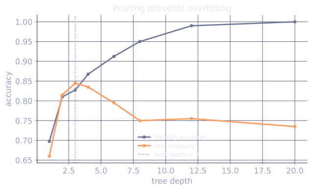
An unconstrained decision tree drives every leaf to zero training error by splitting on noise. The cure is regularization: either pre-pruning (limit the tree as it grows) or post-pruning (build a deep tree, then trim it back). Both inject the bias-variance dial that turns trees into useful learners.

Pre-pruning: stopping rules

Stop splitting a node when any of the following triggers:

• Max depth reached.
• Node has fewer than $n_{\min}$ examples.
• Best split's impurity reduction is below a threshold.
• Best split would create a child smaller than $\ell_{\min}$ examples.

Pre-pruning is simple and cheap. The downside is horizon effect: a poor split early on can prevent a great split later that the algorithm never sees.

Post-pruning: cost-complexity pruning

Grow a deep tree $T_0$, then trim it by minimizing a regularized objective:

where $R(T)$ is the training loss (misclassification rate or MSE), $|T|$ is the number of leaves, and $\alpha \ge 0$ is a complexity cost per leaf.

For each $\alpha$ there is a unique smallest subtree minimizing $R_\alpha$; increasing $\alpha$ from $0$ to $\infty$ generates a nested sequence of subtrees $T_0 \supset T_1 \supset \cdots \supset T_K = \{\text{root}\}$ (weakest-link pruning). Cross-validation picks the $\alpha$ (equivalently the subtree) with the best held-out performance.

This is CART's cost-complexity pruning[1], and it tends to outperform pre-pruning because it considers the full tree before deciding what to keep[2].

Practical hyperparameters

Most production tree implementations expose:

• max_depth (depth cap),
• min_samples_split (refuse to split nodes smaller than this),
• min_samples_leaf (every leaf must be at least this big),
• min_impurity_decrease (gain threshold),
• ccp_alpha (cost-complexity penalty for post-pruning).

A typical grid search varies max_depth and min_samples_leaf first; reach for ccp_alpha when the bias-variance balance is still off.

Single tree vs ensemble

A well-regularized single tree is interpretable but not state-of-the-art. Random forests and gradient boosting (later lessons) use many lightly regularized trees and average them, which reduces variance without paying for the interpretability of each tree.

Check it on arrays

import numpy as np

rng = np.random.default_rng(0)

n = 300
X = rng.uniform(-3, 3, size=(n, 2))
y_clean = (X[:, 0] + X[:, 1] > 0).astype(int)
flip = rng.random(n) < 0.10
y = np.where(flip, 1 - y_clean, y_clean)              # 10% label noise

def gini(labels):
    if len(labels) == 0: return 0.0
    p = np.bincount(labels) / len(labels)
    return 1 - np.sum(p**2)

class Node:
    def __init__(self): self.leaf = None; self.feature = self.threshold = self.left = self.right = None

def split(X, y):
    best = (None, None, -1)
    parent = gini(y); n = len(y)
    for j in range(X.shape[1]):
        for t in np.unique(X[:, j]):
            m = X[:, j] <= t
            if m.sum() == 0 or (~m).sum() == 0: continue
            gain = parent - (m.sum() / n) * gini(y[m]) - ((~m).sum() / n) * gini(y[~m])
            if gain > best[2]: best = (j, t, gain)
    return best

def build(X, y, max_depth=None, min_samples_leaf=1):
    node = Node()
    if max_depth == 0 or len(y) < 2 * min_samples_leaf or gini(y) == 0:
        node.leaf = int(np.argmax(np.bincount(y))); return node
    j, t, gain = split(X, y)
    if j is None or gain <= 0:
        node.leaf = int(np.argmax(np.bincount(y))); return node
    m = X[:, j] <= t
    if m.sum() < min_samples_leaf or (~m).sum() < min_samples_leaf:
        node.leaf = int(np.argmax(np.bincount(y))); return node
    node.feature, node.threshold = j, t
    node.left = build(X[m], y[m], None if max_depth is None else max_depth - 1, min_samples_leaf)
    node.right = build(X[~m], y[~m], None if max_depth is None else max_depth - 1, min_samples_leaf)
    return node

def predict(node, x):
    while node.leaf is None:
        node = node.left if x[node.feature] <= node.threshold else node.right
    return node.leaf

def count_leaves(t): return 1 if t.leaf is not None else count_leaves(t.left) + count_leaves(t.right)

# Train/test split
idx = rng.permutation(n)
tr, te = idx[:200], idx[200:]
Xtr, ytr = X[tr], y[tr]
Xte, yte = X[te], y[te]

# Sweep max_depth: deep tree overfits noise
print(f"{'depth':>6}  {'leaves':>6}  {'train acc':>10}  {'test acc':>10}")
for d in [1, 2, 4, 8, None]:
    T = build(Xtr, ytr, max_depth=d, min_samples_leaf=1)
    tr_acc = np.mean([predict(T, x) for x in Xtr] == ytr)
    te_acc = np.mean([predict(T, x) for x in Xte] == yte)
    print(f"{str(d):>6}  {count_leaves(T):>6}  {tr_acc:>10.3f}  {te_acc:>10.3f}")

Deep trees achieve near-perfect training accuracy but lose on the test set; the shallow tree, with far fewer leaves, generalizes better.

Exercises

Exercise 1. A grown tree $T_0$ has 8 leaves and a training misclassification rate $R(T_0) = 0.05$. A pruned subtree $T_1$ has 5 leaves and $R(T_1) = 0.08$. Using $R_\alpha(T) = R(T) + \alpha\,|T|$, find the value of $\alpha$ at which the two trees have equal cost, and state which tree the objective prefers above and below that $\alpha$.

Exercise 2. The lesson names the horizon effect as the weakness of pre-pruning. Construct a small concrete target where a min-impurity-decrease stop rule prunes a node that a later split would have made highly informative, and explain why post-pruning avoids the trap.

Exercise 3 (code). Implement weakest-link cost-complexity selection on a two-candidate choice: given the grown tree's leaf count and loss and a pruned subtree's leaf count and loss, sweep $\alpha$ over a grid and report the smallest $\alpha$ at which the pruned subtree is preferred. Confirm it matches Exercise 1.

import numpy as np

# (loss, leaves) for the grown tree T0 and the pruned subtree T1
R0, n0 = 0.05, 8
R1, n1 = 0.08, 5

def cost(R, n_leaves, alpha):
    return R + alpha * n_leaves

alphas = np.linspace(0, 0.05, 5001)
prefers_pruned = np.array([cost(R1, n1, a) <= cost(R0, n0, a) for a in alphas])
alpha_star = alphas[np.argmax(prefers_pruned)]   # first True on the grid

# Closed-form crossover from Exercise 1
crossover = (R1 - R0) / (n0 - n1)
assert np.isclose(alpha_star, crossover, atol=1e-3)
print(f"grid alpha*: {alpha_star:.4f}, closed-form crossover: {crossover:.4f}")

The next lesson exploits this variance directly: average many bootstrap-resampled trees to get a Random Forest.

References

- [1]Breiman, L., Friedman, J., Olshen, R., & Stone, C. (1984). Classification and Regression Trees. Wadsworth. Weakest-link cost-complexity pruning of an over-grown tree.↩
- [2]Hastie, T., Tibshirani, R., & Friedman, J. (2009). The Elements of Statistical Learning (2nd ed.). Springer. Tree size selection and pruning (doi:10.1007/978-0-387-84858-7).↩