Normalizing flows

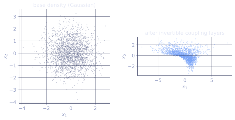
A normalizing flow transforms a simple base distribution (a Gaussian) into the data distribution through a sequence of invertible neural network layers. Because each layer is invertible and has a tractable Jacobian determinant, the exact log-likelihood of any data point can be computed via the change-of-variables formula[1]. This makes flows a clean middle ground between VAEs (likelihood lower bound) and GANs (no likelihood).

The change-of-variables formula

For an invertible $f: \mathbb{R}^d \to \mathbb{R}^d$ and $z = f^{-1}(x)$,

If $f$ is a composition $f = f_L \circ \cdots \circ f_1$ of invertible layers, the log-likelihood becomes a sum:

Train by maximizing $\sum_i \log p_X(x_i)$: a clean negative log-likelihood that gives exact density estimates.

The design challenge

Two competing requirements:

• Expressiveness: each layer must be flexible enough to compose into rich distributions.
• Tractability: each layer must be invertible and have a computable Jacobian determinant.

The full Jacobian is $d \times d$ ($d$ in the thousands for images), so computing its determinant naively is $O(d^3)$. Flow architectures use special structures that make the determinant cheap.

Coupling layers (RealNVP)

Dinh et al. (2017). Split the input into two halves $x = (x_a, x_b)$ and apply[2]:

The first half passes through unchanged; the second half is elementwise-scaled and shifted by functions of the first half. The inverse is

The Jacobian is triangular, so its determinant is the product of the diagonal entries: $\det = \prod_i \exp(s(x_a)_i)$. The log determinant is just $\sum s_i$, computed in $O(d)$.

That single number $\log|\det J| = \sum_i s_i$ is the local volume change the layer applies, and reading it on a scale makes the change-of-variables bookkeeping concrete:

• $\sum s_i = 0$: the layer is locally volume-preserving, factor $e^0 = 1$. A unit cube of latent space maps to a unit cube of data space, density unchanged.
• $\sum s_i = +2$: the map stretches volume by $e^2 \approx 7.4\times$. Density spreads over $7.4$ times the volume, so $p_X$ drops by that factor where the flow expands.
• $\sum s_i = -2$: the map compresses volume to $e^{-2} \approx 0.135\times$. Probability piles up, density rises about $7.4$-fold.

A flow builds a sharp data distribution out of a smooth Gaussian by accumulating these per-layer volume changes; the closing code's stacked layers report log-dets in the range $[-0.28,\ 0.34]$ for this small affine example, each a near-unit volume tweak that compounds across the stack.

Stack many coupling layers, alternating which half is "active", and you get an expressive flow. RealNVP was the first practical normalizing-flow generative model.

Other flow architectures

• Glow (Kingma & Dhariwal, 2018): RealNVP plus invertible 1×1 convolutions and ActNorm. Improved image generation.
• Autoregressive flows (MAF, IAF): $y_i$ depends only on $x_{<i}$ via a masked autoregressive network. Triangular Jacobian, tractable.
• Spline flows: replace affine couplings with monotonic spline transformations. More expressive per layer.
• Continuous flows (NeuralODE, FFJORD): parameterize the transformation as the solution of an ODE; use adjoint methods for gradients. Foundation for flow matching (later D4 lesson).

What flows are good at

• Exact likelihood: no variational bound, no MCMC. Useful for density estimation, anomaly detection, model comparison.
• Invertibility: encode and decode any point, useful for latent manipulation.
• Stable training: maximum likelihood is a simple, well-conditioned objective.

What they are not great at

• Sample quality: at the same parameter count, flows produce worse images than VAEs, GANs, or diffusion. The architectural constraint (invertibility) is restrictive.
• High-dimensional efficiency: the invertibility requirement keeps the data and latent dimensions equal, so you cannot compress.

Flows are a poor choice for state-of-the-art image generation but remain useful for:

• Density estimation in scientific applications (physics, biology).
• Variational inference (use a flow as the variational posterior).
• Building blocks in larger pipelines (e.g., flow-based VAE posteriors).
• The conceptual foundation for flow matching (D4 final lesson), which dropped the invertibility constraint and became state-of-the-art.

Check it on arrays

import numpy as np

rng = np.random.default_rng(0)

# RealNVP-style coupling layer in 1D pairs
def coupling_forward(x, s_fn, t_fn):
    """Split x in half, transform the second half conditioned on the first."""
    d = x.shape[1]
    h = d // 2
    x_a = x[:, :h]; x_b = x[:, h:]
    s = s_fn(x_a); t = t_fn(x_a)
    y_a = x_a
    y_b = x_b * np.exp(s) + t
    log_det = s.sum(axis=1)
    return np.column_stack([y_a, y_b]), log_det

def coupling_inverse(y, s_fn, t_fn):
    d = y.shape[1]
    h = d // 2
    y_a = y[:, :h]; y_b = y[:, h:]
    s = s_fn(y_a); t = t_fn(y_a)
    x_a = y_a
    x_b = (y_b - t) * np.exp(-s)
    return np.column_stack([x_a, x_b])

# Simple s and t: linear functions of the active half
d = 4
W_s = rng.normal(scale=0.3, size=(d // 2, d // 2))
W_t = rng.normal(scale=0.3, size=(d // 2, d // 2))
def s_fn(x): return np.tanh(x @ W_s)                  # bounded for stability
def t_fn(x): return x @ W_t

# Forward and inverse should round-trip
X = rng.normal(size=(10, d))
Y, log_det = coupling_forward(X, s_fn, t_fn)
X_back = coupling_inverse(Y, s_fn, t_fn)
print(f"forward-inverse roundtrip error: {np.max(np.abs(X - X_back)):.2e}")
print(f"log |det J| per sample: {log_det[:5].round(3)}")

# Stack multiple coupling layers, alternating the split (here just two)
def stack_forward(x, layers):
    logdet_total = np.zeros(len(x))
    for s, t in layers:
        x, ld = coupling_forward(x, s, t)
        logdet_total += ld
        # swap halves
        x = np.column_stack([x[:, d//2:], x[:, :d//2]])
    return x, logdet_total

layers = [(s_fn, t_fn), (s_fn, t_fn), (s_fn, t_fn)]
Z, log_det = stack_forward(X, layers)

# log p(x) = log p(z) + log|det df^{-1}/dx|  (stack_forward is the data->latent map)
log_pz = -0.5 * np.sum(Z**2, axis=1) - 0.5 * d * np.log(2 * np.pi)
log_px = log_pz + log_det
print(f"log p(x) for a few samples: {log_px[:5].round(3)}")

Each coupling layer is invertible and contributes a cheap log-Jacobian to the total log-density.

Exercises

Exercise 1. A RealNVP coupling layer sets $y_a = x_a$ and $y_b = x_b \odot \exp(s(x_a)) + t(x_a)$. Show that the Jacobian $\partial y / \partial x$ is lower triangular and that $\log|\det J| = \sum_i s(x_a)_i$.

Exercise 2. A flow stacks layers $f = f_L \circ \cdots \circ f_1$. Starting from the single-step change-of-variables formula, derive the additive log-density $\log p_X(x) = \log p_Z(z_L) + \sum_{\ell=1}^L \log|\det \partial f_\ell / \partial z_{\ell-1}|$, where $z_0 = x$ is mapped to $z_L$ in the base space.

Exercise 3 (code). Implement a 1-D affine flow $z = f(x) = (x - t)\,e^{-s}$ that maps data to a standard normal base, with scalar parameters $s, t$. Use change of variables to evaluate $\log p_X(x)$ and confirm it integrates to a proper density by checking it matches the implied Gaussian $\mathcal{N}(t, e^{2s})$ numerically.

import numpy as np

rng = np.random.default_rng(0)

s, t = 0.4, 1.5                          # flow params: scale e^s, shift t

def f(x):                                # data -> base
    return (x - t) * np.exp(-s)

def log_px(x):
    z = f(x)
    log_pz = -0.5 * z**2 - 0.5 * np.log(2 * np.pi)   # N(0,1) base
    log_det = -s                                      # d/dx of (x - t) e^{-s}
    return log_pz + log_det

# f pushes data to N(0,1), so X = t + e^s * Z is N(t, e^{2s})
xs = np.linspace(-4, 7, 1000)
implied_mu, implied_sigma = t, np.exp(s)
log_gauss = -0.5 * ((xs - implied_mu) / implied_sigma)**2 - np.log(implied_sigma * np.sqrt(2 * np.pi))

print(f"max |log_px - log N(t, e^2s)|: {np.max(np.abs(log_px(xs) - log_gauss)):.2e}")

# numerical normalization: density integrates to 1
px = np.exp(log_px(xs))
integral = np.trapz(px, xs)
print(f"integral of p_X over the grid: {integral:.4f}")

assert np.allclose(log_px(xs), log_gauss, atol=1e-10)
assert np.isclose(integral, 1.0, atol=1e-3)

The next lesson covers the generative method that took over from GANs: diffusion models.