Generative adversarial networks

A generative adversarial network (GAN) trains two networks at war: a generator tries to produce samples that look like real data, and a discriminator tries to tell real from fake. The equilibrium of the game is a generator that matches the data distribution. GANs dominated image generation from 2014 to 2021 and remain useful where sample quality matters and speed matters more than likelihood.

The minimax game

Goodfellow et al. (2014). Generator $G_\theta: \mathcal{Z} \to \mathcal{X}$ maps random noise $z \sim p(z)$ to samples[1]; discriminator $D_\phi: \mathcal{X} \to [0, 1]$ assigns probability that an input is real. The objective:

The discriminator maximizes its log-likelihood of correctly classifying real vs fake; the generator minimizes the discriminator's success.

At the unique optimum:

• $D^\star(x) = p_{\text{data}}(x) / (p_{\text{data}}(x) + p_g(x))$.
• $p_g = p_{\text{data}}$ when this is achievable.

The proof is short: substitute $D^\star$ back into the objective; what remains is the Jensen-Shannon divergence between data and model distributions, minimized when they are equal.

Training procedure

Alternate updates:

1. Sample a batch of real data $\{x_i\}$ and a batch of noise $\{z_i\}$.
2. Discriminator step: compute the loss using both real and fake samples; update $\phi$.
3. Generator step: sample new noise; compute the loss using only fake samples; update $\theta$.
4. Repeat.

In practice the generator is trained with the non-saturating loss $-\log D(G(z))$ instead of $\log(1 - D(G(z)))$. The original form saturates when the discriminator is winning (gradient vanishes); the non-saturating form has stronger gradient early in training.

Mode collapse

The pathological failure mode of GAN training: the generator finds a single (or a few) modes that fool the discriminator and produces only those, ignoring the rest of the data distribution.

Causes:

• The minimax game has saddle points where the generator can stably produce limited variety.
• The discriminator can't always tell "you're missing modes" because it only sees one batch at a time.

Mitigations:

• Minibatch discrimination: discriminator sees a batch and looks at diversity across samples.
• Spectral normalization, gradient penalty: improve discriminator training stability.
• Diverse architectures: BigGAN, StyleGAN have specific architectural choices that resist collapse.

Wasserstein GAN

Arjovsky et al. (2017). Replace the JS-divergence-based loss with the Wasserstein distance (Earth Mover's distance)[2]:

The 1-Lipschitz constraint on $D$ is enforced via weight clipping (WGAN) or gradient penalty (WGAN-GP).

Why it helps: the JS divergence saturates when distributions don't overlap, giving no gradient. The Wasserstein distance always has a useful gradient. Training is more stable, and the discriminator loss correlates with sample quality (useful for monitoring).

DCGAN

Radford et al. (2015). The first practical recipe for stable image GAN training:

• Generator: stack of transposed convolutions with BatchNorm and ReLU.
• Discriminator: stack of strided convolutions with BatchNorm and LeakyReLU.
• No fully connected layers except at the bottleneck.
• Tanh output for the generator (matching $x \in [-1, 1]$).

DCGAN demonstrated that GANs could produce coherent natural images and enabled the field to scale up.

Evaluation

GANs don't have a likelihood, so evaluation is tricky:

• Inception Score (IS): based on a pretrained classifier; rewards confident, diverse classifications. Known to be flawed.
• Fréchet Inception Distance (FID): compute feature statistics for real and generated samples in Inception space; report the Fréchet distance. Standard metric for image GANs.
• Precision and recall: separate fidelity (precision) from diversity (recall).
• Human evaluation: ultimately the gold standard for visual quality.

What killed GANs (for a while)

Diffusion models surpassed GANs on most image-generation benchmarks around 2021-2022. The pure-GAN line lost the lead, although:

• Training-time efficiency: GANs sample in one forward pass; diffusion needs many.
• Latent space structure: StyleGAN's latents are exceptionally manipulable.
• Combined methods: many state-of-the-art image models use adversarial losses together with diffusion or autoencoder losses (e.g., consistency models, VQ-GAN).

GANs are not dead; they're a tool in a larger toolbox.

Check it on arrays

import numpy as np

rng = np.random.default_rng(0)

# 1D toy: real data is a mixture of two Gaussians at -2 and +2
def real_data(n): return np.concatenate([rng.normal(-2, 0.3, n // 2), rng.normal(2, 0.3, n // 2)])

# Tiny generator: z -> linear -> output. Tiny discriminator: x -> linear -> sigmoid.
d_z = 4
W_g1 = rng.normal(scale=0.3, size=(d_z, 8))
W_g2 = rng.normal(scale=0.3, size=(8, 1))
W_d1 = rng.normal(scale=0.3, size=(1, 8))
W_d2 = rng.normal(scale=0.3, size=(8, 1))

def relu(x): return np.maximum(0, x)
def sigmoid(z): return 1 / (1 + np.exp(-z))

def G(z): return relu(z @ W_g1) @ W_g2
def D(x): return sigmoid(relu(x[:, None] @ W_d1) @ W_d2).ravel()

def disc_loss(real, fake):
    return -(np.log(D(real) + 1e-8) + np.log(1 - D(fake) + 1e-8)).mean()

def gen_loss(fake):
    return -np.log(D(fake) + 1e-8).mean()

# Show initial discriminator behavior on real vs fake samples
n_batch = 64
x_real = real_data(n_batch)
z = rng.normal(size=(n_batch, d_z))
x_fake = G(z).ravel()

print(f"discriminator D(real) average: {D(x_real).mean():.3f}")
print(f"discriminator D(fake) average: {D(x_fake).mean():.3f}")
print(f"discriminator loss: {disc_loss(x_real, x_fake):.3f}")
print(f"generator loss:     {gen_loss(x_fake):.3f}")
print(f"fake-sample range: [{x_fake.min():.2f}, {x_fake.max():.2f}]")
print(f"real-sample range: [{x_real.min():.2f}, {x_real.max():.2f}]")

The discriminator initially has near-random output, the generator produces noise; training would alternate updates until $D$ cannot distinguish $G(z)$ from real data.

Exercises

Exercise 1. At a fixed generator, the discriminator maximizes $V = \mathbb{E}_{x\sim p_{\text{data}}}[\log D(x)] + \mathbb{E}_{x\sim p_g}[\log(1 - D(x))]$. Derive the optimal discriminator $D^\star(x) = p_{\text{data}}(x)/(p_{\text{data}}(x) + p_g(x))$ by maximizing the integrand pointwise.

Exercise 2. Substitute $D^\star$ back into $V$ and show the generator then minimizes $2\, D_{\text{JS}}(p_{\text{data}}\,\|\,p_g) - \log 4$, where $D_{\text{JS}}$ is the Jensen-Shannon divergence. Conclude the minimum is at $p_g = p_{\text{data}}$.

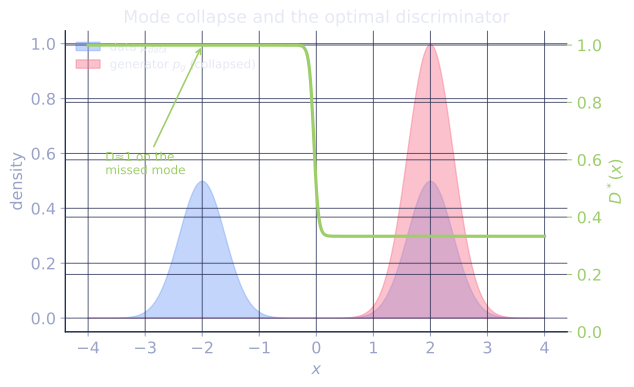
Exercise 3 (code). With both distributions known, the optimal discriminator is computable in closed form. On the lesson's two-Gaussian data and a mode-collapsed generator that covers only the right mode, evaluate $D^\star$ and confirm it stays near $1$ on the abandoned left mode, the gradient signal that should pull the generator to cover it.

import numpy as np

def gauss(x, mu, sd):
    return np.exp(-0.5 * ((x - mu) / sd)**2) / (sd * np.sqrt(2 * np.pi))

# Data: equal mixture of N(-2, 0.3) and N(+2, 0.3)
def p_data(x):
    return 0.5 * gauss(x, -2, 0.3) + 0.5 * gauss(x, 2, 0.3)

# Mode-collapsed generator: only the right mode N(+2, 0.3)
def p_g(x):
    return gauss(x, 2, 0.3)

def D_star(x):
    pd, pg = p_data(x), p_g(x)
    return pd / (pd + pg)

x_left = np.array([-2.0])           # abandoned mode
x_right = np.array([2.0])           # covered mode
print(f"D*(-2) on abandoned mode: {D_star(x_left)[0]:.4f}")
print(f"D*(+2) on covered mode:   {D_star(x_right)[0]:.4f}")

assert D_star(x_left)[0] > 0.99     # near 1: generator missing this mode
assert np.isclose(D_star(x_right)[0], 1/3, atol=1e-2)   # p_g = 2*p_data here

The next lesson surveys the production GAN families: DCGAN, StyleGAN, BigGAN.

References

- [1]Goodfellow, I., et al. (2014). "Generative adversarial nets". NeurIPS. arXiv:1406.2661. The minimax game and the JS-divergence optimum.↩
- [2]Arjovsky, M., Chintala, S., & Bottou, L. (2017). "Wasserstein GAN". ICML. arXiv:1701.07875. The Wasserstein objective and its non-vanishing gradient.↩