Diffusion models

Diffusion models are the dominant generative paradigm of the 2020s. The recipe: add Gaussian noise to data in many small steps (the forward process), then learn to reverse the noising step by step. At inference, start from pure noise and denoise to a clean sample. The math is clean (variational like a VAE, hierarchical with shared parameters), the training is stable, and the samples are state-of-the-art across images, audio, and video.

The forward process

Given a data sample $x_0$, define a sequence $x_0, x_1, \dots, x_T$ by gradually adding Gaussian noise:

with noise schedule $\beta_t \in (0, 1)$. The marginals have a closed form:

where $\alpha_t = 1 - \beta_t$ and $\bar\alpha_t = \prod_{s=1}^t \alpha_s$. By $T \approx 1000$ steps with a reasonable schedule, $\bar\alpha_T \approx 0$, and $x_T$ is nearly pure noise.

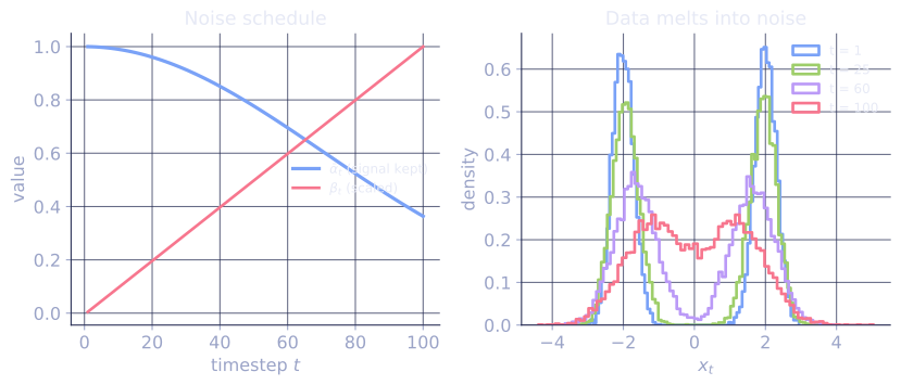
The single number $\bar\alpha_t$ controls the signal-to-noise mix at step $t$: the clean sample enters with weight $\sqrt{\bar\alpha_t}$ and the noise with weight $\sqrt{1 - \bar\alpha_t}$. On the standard linear schedule ($T = 1000$, $\beta_t$ from $10^{-4}$ to $0.02$) those weights trace the whole range. At $t = 1$, $\bar\alpha_t \approx 0.9999$: signal weight $\approx 1.000$, noise weight $\approx 0.010$, the image barely perturbed. At $t = 500$, $\bar\alpha_t \approx 0.079$: signal $\approx 0.28$, noise $\approx 0.96$, half-melted. At $t = 1000$, $\bar\alpha_t \approx 4 \times 10^{-5}$: signal $\approx 0.006$, noise $\approx 1.000$, indistinguishable from a draw of $\mathcal{N}(0, I)$. The schedule is just this monotone slide from all-signal to all-noise.

A key reparameterization:

So at any timestep, $x_t$ is a known interpolation between $x_0$ and random noise.

The reverse process

The forward process is fixed; the reverse process is learned:

To sample, start at $x_T \sim \mathcal{N}(0, I)$ and apply the learned reverse step $T$ times: $x_T \to x_{T-1} \to \dots \to x_0$.

For Gaussian $q$ with small steps, the reverse process is also nearly Gaussian. The model just needs to predict the mean (and optionally the variance).

The DDPM objective

Ho et al. (2020). After algebra on the ELBO, the training objective reduces to a stunningly simple form[1]:

The model $\epsilon_\theta$ takes a noisy sample $x_t$ and the timestep $t$ and predicts the noise that was added. Training:

1. Sample a clean data point $x_0$.
2. Sample a timestep $t \sim \operatorname{Uniform}(1, T)$.
3. Sample noise $\epsilon \sim \mathcal{N}(0, I)$.
4. Compute $x_t = \sqrt{\bar\alpha_t}\, x_0 + \sqrt{1 - \bar\alpha_t}\,\epsilon$.
5. Loss: $\lVert \epsilon - \epsilon_\theta(x_t, t)\rVert^2$.

Why it works: the noise prediction task is well-posed across timesteps (easy when $t$ is small, hard when $t$ is large), and the model gets a diverse curriculum of noise levels by sampling $t$ uniformly.

Sampling (DDPM)

Given the learned $\epsilon_\theta$:

with $z \sim \mathcal{N}(0, I)$. Iterate from $t = T$ down to $t = 1$.

The reverse step takes the current noisy sample, predicts the noise to remove, and applies that estimate plus a smaller amount of fresh noise (except at $t = 1$).

A typical $T$ is 1000 for DDPM, meaning 1000 forward passes per sample. This is slow; the next sections cover faster samplers.

DDIM and other faster samplers

Song et al. (2021). DDIM generalizes the sampling step:

where $\hat x_0 = (x_t - \sqrt{1 - \bar\alpha_t}\,\epsilon_\theta)/\sqrt{\bar\alpha_t}$ is the predicted clean sample.

When $\sigma_t = 0$, the process becomes deterministic, and you can skip many timesteps without losing quality. DDIM can sample in 10-50 steps instead of 1000.

Newer samplers (DPM-Solver, EDM, consistency distillation) push this further to 1-8 steps per sample.

What the model actually learns

The denoiser $\epsilon_\theta(x_t, t)$ is implicitly the score function of the noisy data:

The score is the gradient of the log-density of the noisy data. The reverse process is then gradient ascent on the noisy log-density: at each step, move in the direction the data is more likely.

This connection (diffusion = score-based generative model) was made rigorous by Song & Ermon and gives a unified view of DDPM and the continuous-time score-based formulation[2].

Conditional generation

For class-conditional or text-conditional generation, concatenate the condition $c$ to the input of the denoiser: $\epsilon_\theta(x_t, t, c)$.

Classifier-free guidance (CFG) is the dominant technique for strengthening conditioning:

where $\emptyset$ is "no condition" (trained by randomly dropping the condition during training). Higher $w$ (typically 7-15) produces sharper, more on-prompt samples at the cost of diversity.

What diffusion gave the field

• Stable training at scale.
• State-of-the-art sample quality on images, audio, and video.
• Strong conditional generation via cross-attention.
• A clean likelihood-bound objective that scales with compute.

The next two lessons cover the productionized form (latent diffusion) and the modern continuous-time generalization (flow matching).

Check it on arrays

import numpy as np

rng = np.random.default_rng(0)

T = 100                                                # diffusion timesteps
beta = np.linspace(1e-4, 0.02, T)                      # linear schedule
alpha = 1.0 - beta
alpha_bar = np.cumprod(alpha)

# Forward process: closed form
def forward(x0, t, rng):
    """Sample x_t given x_0 and timestep t (1-indexed)."""
    eps = rng.normal(size=x0.shape)
    return np.sqrt(alpha_bar[t - 1]) * x0 + np.sqrt(1 - alpha_bar[t - 1]) * eps, eps

# 1D toy: data is mixture of two Gaussians
x0 = np.concatenate([rng.normal(-2, 0.3, 500), rng.normal(2, 0.3, 500)])
print("forward process: noise grows with t")
for t in [1, 25, 50, 75, 100]:
    xt, _ = forward(x0, t, rng)
    print(f"  t={t:>3}: x_t mean={xt.mean():+.3f}, std={xt.std():.3f}")

# A perfect denoiser would output the true epsilon; here mock with a learned-fit
# Fit a tiny linear "denoiser" that maps x_t to noise: epsilon_pred = a * x_t + b
A = np.zeros(T); B = np.zeros(T)
for t in range(1, T + 1):
    xt, eps = forward(x0, t, rng)
    # OLS for one-dim eps = a * x + b
    a = np.cov(xt, eps)[0, 1] / np.var(xt)
    b = eps.mean() - a * xt.mean()
    A[t - 1] = a; B[t - 1] = b

# DDPM sampling from this naive denoiser
def sample(n, A, B, rng):
    x = rng.normal(size=n)                              # start from N(0, 1)
    for t in range(T, 0, -1):
        eps_pred = A[t - 1] * x + B[t - 1]
        mu = (x - beta[t - 1] / np.sqrt(1 - alpha_bar[t - 1]) * eps_pred) / np.sqrt(alpha[t - 1])
        if t > 1:
            x = mu + np.sqrt(beta[t - 1]) * rng.normal(size=n)
        else:
            x = mu
    return x

samples = sample(2000, A, B, rng)
print(f"\nsampled distribution: mean={samples.mean():.3f}, std={samples.std():.3f}")
print(f"true data:           mean={x0.mean():.3f}, std={x0.std():.3f}")

The forward process visibly noisifies the data; the naive linear denoiser plus DDPM sampling recovers a sample distribution close to the original.

Exercises

Exercise 1. The forward process is $q(x_t \mid x_{t-1}) = \mathcal{N}(\sqrt{1 - \beta_t}\, x_{t-1},\ \beta_t I)$ with $\alpha_t = 1 - \beta_t$. Show that the marginal given $x_0$ is $q(x_t \mid x_0) = \mathcal{N}(\sqrt{\bar\alpha_t}\, x_0,\ (1 - \bar\alpha_t) I)$ with $\bar\alpha_t = \prod_{s=1}^t \alpha_s$, by composing two steps and inducting.

Exercise 2. On the standard linear schedule ($T = 1000$, $\beta_t$ from $10^{-4}$ to $0.02$), compute the signal weight $\sqrt{\bar\alpha_t}$ and noise weight $\sqrt{1 - \bar\alpha_t}$ at $t = 1$ and verify they match the lesson's quoted $\approx 1.000$ and $\approx 0.010$.

Exercise 3 (code). Implement one forward noising step in closed form and confirm it empirically. Draw many samples of $x_t = \sqrt{\bar\alpha_t}\, x_0 + \sqrt{1 - \bar\alpha_t}\,\epsilon$ for a fixed $x_0$ and check the sample mean and variance match $\sqrt{\bar\alpha_t}\, x_0$ and $1 - \bar\alpha_t$.

import numpy as np

rng = np.random.default_rng(0)

T = 1000
beta = np.linspace(1e-4, 0.02, T)
alpha = 1.0 - beta
alpha_bar = np.cumprod(alpha)

t = 500                                   # 1-indexed timestep
ab = alpha_bar[t - 1]
x0 = 1.3                                   # fixed clean scalar

N = 2_000_000
eps = rng.normal(size=N)
xt = np.sqrt(ab) * x0 + np.sqrt(1 - ab) * eps    # closed-form forward step

mean_emp, var_emp = xt.mean(), xt.var()
mean_true, var_true = np.sqrt(ab) * x0, 1 - ab
print(f"t={t}: alpha_bar={ab:.4f}")
print(f"mean  empirical {mean_emp:.4f}  true {mean_true:.4f}")
print(f"var   empirical {var_emp:.4f}  true {var_true:.4f}")

assert np.isclose(mean_emp, mean_true, atol=2e-3)
assert np.isclose(var_emp, var_true, atol=2e-3)

The next lesson moves to the production form: latent diffusion (Stable Diffusion).

References

- [1]Ho, J., Jain, A., & Abbeel, P. (2020). "Denoising diffusion probabilistic models (DDPM)". NeurIPS. arXiv:2006.11239. The noise-prediction objective and DDPM sampling.↩
- [2]Song, Y., & Ermon, S. (2019). "Generative modeling by estimating gradients of the data distribution". NeurIPS. arXiv:1907.05600. Score matching across noise levels, the score-based view of denoising.↩