Variational autoencoders

The plain autoencoder learns a useful bottleneck but its latent space is unstructured: sampling random codes gives garbage. The variational autoencoder (VAE) adds a probabilistic structure: each input maps to a distribution over latents, and a prior keeps that distribution well-behaved. Sampling becomes principled, the model has a likelihood, and the math (the ELBO) generalizes to a huge family of latent-variable models[1].

The generative story

A VAE assumes data comes from a two-step process:

1. Sample a latent $z \sim p(z)$ from a simple prior (typically $\mathcal{N}(0, I)$).
2. Sample $x \sim p_\theta(x \mid z)$ from a decoder distribution.

The data likelihood is $p_\theta(x) = \int p_\theta(x \mid z)\, p(z)\, dz$. The integral is intractable for any interesting decoder, so we cannot maximize $\log p_\theta(x)$ directly.

The ELBO

Introduce an approximate posterior $q_\phi(z \mid x)$ produced by an encoder. By the standard variational identity:

The last KL is non-negative, so

This is the evidence lower bound (ELBO). Maximize it (equivalently, minimize its negation) jointly over $\theta$ and $\phi$.

The two terms have intuitive readings:

• Reconstruction term: the decoder should make $x$ likely given $z$ sampled from the encoder. For a Gaussian decoder, this becomes $-\lVert x - g_\theta(z)\rVert^2$, the same as the plain autoencoder.
• KL term: the encoder distribution should stay close to the prior. This prevents the encoder from collapsing to delta functions (which would maximize reconstruction but make the latent space useless).

Gaussian encoder

The standard choice: $q_\phi(z \mid x) = \mathcal{N}(\mu_\phi(x),\ \operatorname{diag}(\sigma_\phi(x)^2))$, with $\mu_\phi$ and $\log \sigma_\phi$ produced by an encoder MLP.

With this choice and standard normal prior $p(z) = \mathcal{N}(0, I)$, the KL has a closed form:

No Monte Carlo estimation needed for the KL.

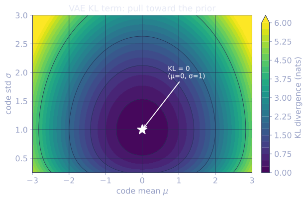
To calibrate what this penalty costs, read it one latent dimension at a time, $\tfrac12(\mu^2 + \sigma^2 - 1 - \log\sigma^2)$:

• $\mu = 0,\ \sigma = 1$: the code already matches the prior, KL $= 0$. No penalty.
• $\mu = 1,\ \sigma = 1$: shifted one standard deviation off-center, KL $= 0.5$ nat. A modest pull back toward the origin.
• $\mu = 2,\ \sigma = 1$: two off-center, KL $= 2$ nats. The cost grows quadratically in the mean.
• $\mu = 0,\ \sigma = 0.1$: centered but the posterior has collapsed to a near delta, KL $\approx 1.81$ nats. The same $\sigma = 0.1$ at $\mu = 3$ costs $\approx 6.31$ nats.

Two ways to drift carry different prices, which is the distinction the loss enforces. A confident-but-centered code ($\mu = 0,\ \sigma = 0.1$) and an uncertain-but-displaced code ($\mu = 1,\ \sigma = 1$) are both off the prior, but the over-confident one costs $1.81$ nats against $0.5$: the KL punishes a posterior that pins $z$ down (small $\sigma$) harder than one that merely sits a step away, which is what keeps the latent space smooth enough to interpolate through.

The reparameterization trick

The reconstruction term requires sampling $z \sim q_\phi(z \mid x)$, which makes the loss non-differentiable in $\phi$ (you can't backprop through a sample).

Reparameterization: write the sample as a deterministic function of $\phi$ and a standard normal noise:

Now $z$ is a differentiable function of $\phi$ (with $\epsilon$ random but treated as input), and backprop flows through the sample. This is the key trick that made VAE training practical[2].

Training procedure

1. Forward: encoder produces $\mu(x), \sigma(x)$; sample $z$ via reparameterization; decoder produces $\hat x$.
2. Loss: reconstruction + KL.
3. Backward: gradient flows through both terms via reparameterization.

Inference (generation): sample $z \sim \mathcal{N}(0, I)$ from the prior, decode. Because the KL term forced the encoder's posterior distributions to stay close to the prior, the prior is the "right" distribution to sample from.

Posterior collapse

A common failure: the decoder is so expressive that it can fit the data without using $z$ at all. The encoder then becomes useless: it outputs the prior regardless of input, the KL term is zero, and the latent encodes nothing.

Symptoms: KL term goes to zero, latent dimensions look like random noise, reconstructions ignore the encoder.

Mitigations:

• KL annealing: scale the KL term up over training (start with 0, end with 1).
• Free bits: only penalize KL above a threshold per dimension.
• Architectural choices: less expressive decoder, autoregressive prior.

What VAEs are good at and not

Good at:

• Smooth, interpretable latent spaces (interpolation works).
• Likelihood estimation (the ELBO is a true bound on log-likelihood).
• Conditional generation when class labels or text are fed to the decoder.
• Building block for many later methods (latent diffusion uses a VAE).

Not as good as:

• Sample quality vs GANs (VAEs produce blurry samples because Gaussian decoders smooth over uncertainty).
• Sample quality vs diffusion (diffusion now dominates both).

VAEs hold up best as a representation-learning backbone and as a component in larger pipelines (e.g., the autoencoder in Stable Diffusion is a VAE).

Check it on arrays

import numpy as np

rng = np.random.default_rng(0)

# 1D toy: data from two well-separated modes
n = 1000
x = np.concatenate([rng.normal(-2, 0.3, n // 2), rng.normal(2, 0.3, n // 2)])

# Simple VAE: encoder produces mu, log_sigma; decoder produces x_hat
d_z, d_h = 2, 16
def init(in_d, out_d): return rng.normal(scale=0.3 / np.sqrt(in_d), size=(in_d, out_d))
W_enc1 = init(1, d_h); b_enc1 = np.zeros(d_h)
W_mu = init(d_h, d_z); b_mu = np.zeros(d_z)
W_logs = init(d_h, d_z); b_logs = np.zeros(d_z)
W_dec1 = init(d_z, d_h); b_dec1 = np.zeros(d_h)
W_dec2 = init(d_h, 1); b_dec2 = np.zeros(1)

def encode(x):
    h = np.maximum(0, x[:, None] @ W_enc1 + b_enc1)
    return h @ W_mu + b_mu, h @ W_logs + b_logs

def decode(z):
    h = np.maximum(0, z @ W_dec1 + b_dec1)
    return (h @ W_dec2 + b_dec2).ravel()

def vae_step(x, lr=0.01, kl_weight=0.5):
    mu, log_sigma = encode(x)
    sigma = np.exp(log_sigma)
    eps = rng.normal(size=mu.shape)
    z = mu + sigma * eps
    xhat = decode(z)
    recon = np.mean((xhat - x)**2)
    kl = 0.5 * np.mean(np.sum(mu**2 + sigma**2 - 1 - 2 * log_sigma, axis=1))
    return recon, kl, mu, sigma, xhat

# Train (single-step, no full backprop) just to check the forward and loss
recon, kl, mu, sigma, xhat = vae_step(x)
print(f"initial ELBO terms: recon = {recon:.3f}, KL = {kl:.3f}")
print(f"latent means range: [{mu.min():.2f}, {mu.max():.2f}]")

# Sampling from the prior and decoding gives synthetic data
z_sample = rng.normal(size=(20, d_z))
x_sample = decode(z_sample)
print(f"sampled from prior, decoded: {x_sample.round(2)[:10]}")

The ELBO splits cleanly into reconstruction and KL; prior samples decode to outputs in the data range (training would push them toward the modes).

Exercises

Exercise 1. Derive the closed-form KL term for one latent dimension. With $q = \mathcal{N}(\mu, \sigma^2)$ and prior $p = \mathcal{N}(0, 1)$, show that $D_{\text{KL}}(q\,\|\,p) = \tfrac12(\mu^2 + \sigma^2 - 1 - \log \sigma^2)$.

Exercise 2. The reparameterization trick rewrites a sample as $z = \mu + \sigma\, \epsilon$ with $\epsilon \sim \mathcal{N}(0, 1)$. For a scalar loss $\ell(z)$, show that the gradient of $\mathbb{E}_{q}[\ell(z)]$ with respect to $\mu$ equals $\mathbb{E}_{\epsilon}[\ell'(z)]$, so the gradient passes through the sample. Contrast this with differentiating the same expectation when the sample is not reparameterized.

Exercise 3 (code). Verify the reparameterized gradient estimator against the analytic gradient. For $\ell(z) = z^2$ and $q = \mathcal{N}(\mu, \sigma^2)$, $\mathbb{E}_q[z^2] = \mu^2 + \sigma^2$, so $\partial/\partial\mu = 2\mu$. Estimate it by sampling $z = \mu + \sigma\epsilon$ and averaging $2z$ (which is $\ell'(z)$), then check it matches $2\mu$.

import numpy as np

rng = np.random.default_rng(0)

mu, sigma = 1.5, 0.7
N = 2_000_000

eps = rng.normal(size=N)
z = mu + sigma * eps                  # reparameterized samples
grad_est = np.mean(2 * z)            # E[l'(z)] with l(z) = z^2, l'(z) = 2z
grad_true = 2 * mu                   # d/dmu of (mu^2 + sigma^2)

print(f"reparam gradient estimate: {grad_est:.4f}   analytic: {grad_true:.4f}")

assert np.isclose(grad_est, grad_true, atol=2e-3)

The next lesson covers VAE variants that improve disentanglement and discrete-latent control.

References

- [1]Kingma, D. P., & Welling, M. (2014). "Auto-encoding variational bayes". ICLR. arXiv:1312.6114. The original VAE: the ELBO and the amortized variational posterior.↩
- [2]Goodfellow, I., Bengio, Y., & Courville, A. (2016). Deep Learning, §20.10.3 (Variational Autoencoders). MIT Press. The reparameterization trick as a path to low-variance gradients.↩