Autoencoders

The simplest generative-style neural network: an autoencoder compresses inputs through a low-dimensional bottleneck and reconstructs them. The reconstruction loss forces the bottleneck to capture whatever structure is useful for reproducing the data[1]. This lesson grounds the generative-modeling track by establishing the encoder-decoder pattern that VAEs and diffusion models will build on[2].

The architecture

An autoencoder has two halves:

• Encoder $f_\phi: \mathcal{X} \to \mathcal{Z}$ maps an input to a low-dimensional latent code $z \in \mathbb{R}^k$.
• Decoder $g_\theta: \mathcal{Z} \to \mathcal{X}$ maps the code back to a reconstruction $\hat x$.

Train end-to-end on the reconstruction loss:

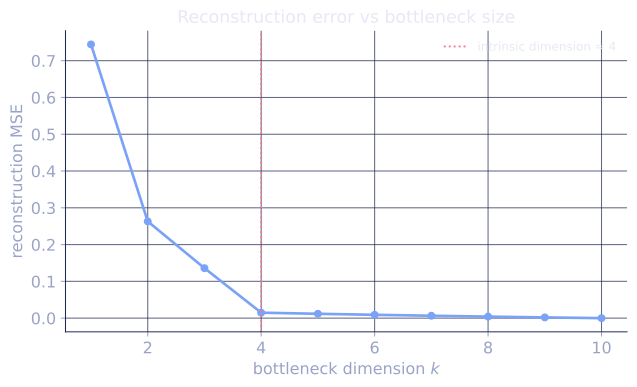
The bottleneck dimension $k$ is the central design choice: small enough that the network cannot just pass the input through, large enough that the structure of the data can be captured.

Linear autoencoder = PCA

When the encoder and decoder are linear and the loss is squared error, the autoencoder reduces to PCA. The optimal encoder is the projection onto the top-$k$ principal components, and the optimal decoder is its transpose. This was the anomaly-detection lesson's setup.

The autoencoder framing matters when the structure is nonlinear: encoder and decoder become MLPs (or CNNs for images), and the latent space can capture curved manifolds that PCA cannot.

What the latent encodes

After training, the latent code captures what the decoder needs to reconstruct $x$:

• Discarded: any input variation the decoder cannot exploit (pure noise, irrelevant detail).
• Kept: anything that systematically helps reconstruction (object identity, pose, color, structural features).

This makes autoencoders useful for representation learning even when generation is not the goal. The latent space often has interpretable structure: similar inputs are nearby, distinct classes occupy distinct regions.

Denoising autoencoder (DAE)

Vincent et al. (2008). Train the autoencoder to reconstruct the clean input from a corrupted version:

where $\tilde x_i$ is $x_i$ with noise added (Gaussian, masked pixels, etc.).

Why corrupt the input? Two reasons:

• Prevents identity learning: an unconstrained autoencoder with a large enough bottleneck can learn the identity function, which is useless. Denoising forces the model to learn the underlying manifold.
• Implicit manifold learning: the model must map corrupted inputs back to the data manifold. The reconstruction error is the "energy" of corruption, and minimizing it teaches the network the shape of the manifold.

The denoising recipe seeded modern generative models:

• Diffusion models are sequences of denoising autoencoders at different noise levels (last lessons in D4).
• Masked autoencoders (MAE) are denoising in the masked-token form for vision (D2 lesson).
• BERT is essentially a masked denoising autoencoder for text.

What autoencoders cannot do

Plain autoencoders are not proper generative models:

• The latent space is unstructured. Sampling a random $z$ and decoding it usually gives garbage, because the encoder has only populated some regions of the latent space.
• There is no notion of likelihood. The model can reconstruct inputs but not generate new ones in a principled way.

The next lesson fixes both with the variational autoencoder, which adds a probabilistic structure to the latent space.

Practical uses (beyond stepping-stone to VAE)

• Dimensionality reduction: replace PCA when nonlinear structure matters (e.g., t-SNE / UMAP precomputation).
• Anomaly detection (C6 lesson): high reconstruction error flags out-of-distribution points.
• Feature extraction: use the encoder's output as features for a downstream classifier.
• Image compression: trained autoencoders can outperform JPEG at low bit rates.

Check it on arrays

import numpy as np

rng = np.random.default_rng(0)

# Synthetic 2D data on a curve in 10D ambient space
n = 500
t = rng.uniform(0, 2 * np.pi, n)
X = np.column_stack([
    np.cos(t), np.sin(t),
    0.5 * np.cos(2 * t), 0.5 * np.sin(2 * t),
    rng.normal(scale=0.05, size=(n, 6))               # noise dims
])
d = X.shape[1]

# Tiny MLP autoencoder: d -> 16 -> 2 -> 16 -> d
def init(in_d, out_d): return rng.normal(scale=0.5 / np.sqrt(in_d), size=(in_d, out_d))
W1 = init(d, 16); b1 = np.zeros(16)
W2 = init(16, 2); b2 = np.zeros(2)
W3 = init(2, 16); b3 = np.zeros(16)
W4 = init(16, d); b4 = np.zeros(d)

def relu(x): return np.maximum(0, x)
def encode(X): return relu(X @ W1 + b1) @ W2 + b2          # signed bottleneck (no ReLU on top)
def decode(z): return relu(z @ W3 + b3) @ W4 + b4
def forward(X): return decode(encode(X))

# Train with SGD on the reconstruction loss
lr = 0.1
for epoch in range(500):
    h_pre = X @ W1 + b1
    h_enc = relu(h_pre)                                    # encoder hidden (post-relu)
    Z = h_enc @ W2 + b2                                    # bottleneck (signed)
    d_pre = Z @ W3 + b3
    d_hid = relu(d_pre)                                    # decoder hidden
    Xhat = d_hid @ W4 + b4
    err = Xhat - X
    # Manual backprop through the chain
    grad_W4 = d_hid.T @ err / n
    grad_b4 = err.mean(axis=0)
    grad_d_pre = (err @ W4.T) * (d_pre > 0)
    grad_W3 = Z.T @ grad_d_pre / n
    grad_b3 = grad_d_pre.mean(axis=0)
    grad_z = grad_d_pre @ W3.T                             # no ReLU on Z, so this is grad wrt Z directly
    grad_W2 = h_enc.T @ grad_z / n
    grad_b2 = grad_z.mean(axis=0)
    grad_h = grad_z @ W2.T
    grad_W1 = X.T @ (grad_h * (h_pre > 0)) / n
    grad_b1 = (grad_h * (h_pre > 0)).mean(axis=0)
    W4 -= lr * grad_W4; b4 -= lr * grad_b4
    W3 -= lr * grad_W3; b3 -= lr * grad_b3
    W2 -= lr * grad_W2; b2 -= lr * grad_b2
    W1 -= lr * grad_W1; b1 -= lr * grad_b1

# Reconstruction quality
Xhat = forward(X)
rmse = np.sqrt(np.mean((Xhat - X)**2))
print(f"autoencoder RMSE on training data: {rmse:.4f}")

# Compare to PCA at the same bottleneck dimension
mean = X.mean(axis=0); Xc = X - mean
U, s, Vt = np.linalg.svd(Xc, full_matrices=False)
V_k = Vt[:2]
X_pca = (Xc @ V_k.T) @ V_k + mean
rmse_pca = np.sqrt(np.mean((X_pca - X)**2))
print(f"PCA k=2 RMSE on the same data:     {rmse_pca:.4f}")

The nonlinear autoencoder beats linear PCA at the same bottleneck because it can model the curved structure.

Exercises

Exercise 1. A linear autoencoder has encoder $f(x) = W x$ and decoder $g(z) = U z$ with $W \in \mathbb{R}^{k \times d}$ and $U \in \mathbb{R}^{d \times k}$, trained on centered data with squared reconstruction error. Show that if $W$ is fixed to the top-$k$ PCA projection $V_k^\top$ (rows orthonormal), the decoder that minimizes reconstruction error is $U = V_k$, so the optimum reconstructs by projecting onto the principal subspace.

Exercise 2. In the denoising autoencoder, the corruption $\tilde x = x + \eta$ with $\eta \sim \mathcal{N}(0, \sigma^2 I)$ is independent of $x$. For a fixed map $g \circ f$, show that the expected denoising loss $\mathbb{E}_{x,\eta}\lVert x - (g \circ f)(x + \eta)\rVert^2$ is minimized, over all measurable maps, by $(g \circ f)(\tilde x) = \mathbb{E}[x \mid \tilde x]$, the posterior mean of the clean input given the corrupted one.

Exercise 3 (code). Build a linear autoencoder with $k = 2$ by hand on 3D data lying near a 2D plane. Confirm that closing the loop with the PCA projection $U = V_k$, $W = V_k^\top$ gives exactly the PCA reconstruction error, matching Exercise 1.

import numpy as np

rng = np.random.default_rng(0)

# 3D data near a 2D plane: two latent directions plus small off-plane noise
n = 400
basis = np.array([[1.0, 0.0, 0.0], [0.0, 1.0, 0.0]])     # spanning plane
coeffs = rng.normal(size=(n, 2)) * np.array([3.0, 1.0])
X = coeffs @ basis + rng.normal(scale=0.05, size=(n, 3))  # off-plane noise on dim 3
X = X - X.mean(axis=0)                                     # center

# PCA: top-2 principal directions
U_svd, s, Vt = np.linalg.svd(X, full_matrices=False)
V_k = Vt[:2].T                                            # d x k, orthonormal cols

# Linear autoencoder with W = V_k^T (encoder), U = V_k (decoder)
W = V_k.T                                                 # k x d
U = V_k                                                   # d x k
Z = X @ W.T                                               # codes
Xhat_ae = Z @ U.T                                         # reconstruction

# Direct PCA reconstruction
Xhat_pca = (X @ V_k) @ V_k.T

err_ae = np.mean(np.sum((X - Xhat_ae)**2, axis=1))
err_pca = np.mean(np.sum((X - Xhat_pca)**2, axis=1))
print(f"linear AE error: {err_ae:.6f}   PCA error: {err_pca:.6f}")

assert np.allclose(Xhat_ae, Xhat_pca)
assert np.isclose(err_ae, err_pca)

The next lesson upgrades this to a proper generative model: the variational autoencoder.

References

- [1]Goodfellow, I., Bengio, Y., & Courville, A. (2016). Deep Learning, §14 (Autoencoders). MIT Press. The encoder-decoder bottleneck and the denoising variant.↩
- [2]Kingma, D. P., & Welling, M. (2014). "Auto-encoding variational bayes". ICLR. arXiv:1312.6114. The variational autoencoder built on the encoder-decoder pattern this lesson establishes.↩