Flow matching and consistency models

DDPM-style discrete diffusion was the breakthrough; flow matching is its cleaner continuous-time successor. Both train a generator by matching a noise-removing field; flow matching has a simpler objective and runs at fewer sampling steps for the same quality. Consistency models push the same generative quality into one or two steps. SD 3, FLUX, and many 2024+ models use these methods as the default.

Continuous-time view of diffusion

DDPM is a discretization of a continuous-time stochastic differential equation:

$$dx_t = f(x_t, t)\, dt + g(t)\, dW_t,$$

where $W$ is Wiener noise. The reverse SDE (or its equivalent ODE) has the form

$$dx_t = [f(x_t, t) - g(t)^2\, \nabla \log p_t(x_t)]\, dt + g(t)\, dW_t.$$

Sampling from data is integrating this reverse-time equation; learning the score $\nabla \log p_t$ is what diffusion does.

The continuous-time view unified DDPM, NCSN, and other score-based methods; flow matching is the next conceptual simplification.

Flow matching

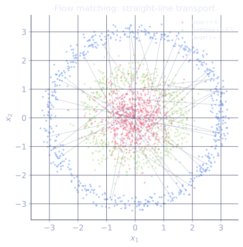
Lipman et al. (2023). Skip the noise/score framing[1]. Define a probability path $p_t(x)$ that interpolates between a simple base $p_0$ (e.g., $\mathcal{N}(0, I)$) and the data distribution $p_1$. Each path has an associated vector field $v_t(x)$ that transports samples along it: a point at time $t$ at position $x$ moves with velocity $v_t(x)$.

Train a neural network $v_\theta(x, t)$ to match the true vector field.

For a Gaussian path (the simplest choice),

$$x_t = (1 - t)\, x_0 + t\, x_1, \qquad x_0 \sim p_0,\ x_1 \sim p_{\text{data}},$$

the conditional vector field is $u_t(x \mid x_1) = x_1 - x_0$. The flow-matching loss is

$$\mathcal{L}_{\text{FM}} = \mathbb{E}_{t, x_0, x_1}\!\left[\lVert v_\theta((1-t)x_0 + t x_1,\ t) - (x_1 - x_0)\rVert^2\right].$$

Compare to DDPM's loss: same shape (predict a target given a noisy input), simpler target (a straight-line direction instead of a noise sample at a specific schedule).

Rectified flow

Liu et al. (2023). The same idea, with iterative rectification[2]: after training a flow $v_\theta$, sample many pairs $(x_0, x_1)$ from the flow by integrating $v_\theta$, then retrain a new flow on these pairs. Each rectification makes the trajectories straighter, reducing the number of sampling steps needed.

A fully rectified flow can sample in 1-2 steps with comparable quality to a 50-step DDPM.

Why flow matching often wins

• Simpler training objective: no noise schedules, no parameterization choices ($v$, $\epsilon$, $x_0$).
• Straighter paths: a Gaussian interpolation produces less curved trajectories than the DDPM noising process, so fewer sampling steps are needed.
• Cleaner conditioning: classifier-free guidance maps straightforwardly.
• Better empirical scaling: matches or beats DDPM-style training at the same parameter count.

SD 3 switched from DDPM to flow matching. FLUX, Pyramid Flow, and many 2024 models followed.

Consistency models

Song et al. (2023). Train a model that directly maps any noisy sample at any timestep to the same final clean sample[3]:

$$f_\theta(x_t, t) = f_\theta(x_{t'}, t')\ \ \text{for all }t, t'.$$

After training, sampling is one network call: $\hat x_0 = f_\theta(x_T, T)$.

Two training routes:

• Consistency distillation: start from a pretrained diffusion model, distill it into a consistency model.
• Consistency training: train from scratch with a loss that enforces the consistency property between adjacent timesteps.

Consistency models have similar quality to many-step diffusion at 1-2 steps. Combined with adversarial losses, they're approaching GAN-level inference speed with diffusion-level quality.

What's next

The generative-modeling landscape as of 2024:

• Flow matching is the dominant training framework for new models.
• Consistency distillation is the dominant deployment technique for fast inference.
• DiTs are replacing U-Nets in the backbone.
• Multimodal extensions (video, 3D, audio) are the active research frontier.

Less than a decade after diffusion's debut, the field has converged on a clean recipe: train a continuous-time flow with a Transformer backbone, distill into a few-step sampler, condition with cross-attention on a strong multimodal text encoder. The next subsection (D5) returns to a different problem: pretraining representations without labels.

Exercises

Exercise 1. For the straight-line Gaussian path $x_t = (1 - t)x_0 + t x_1$ with endpoints $x_0 \sim p_0$, $x_1 \sim p_{\text{data}}$, derive the conditional vector field $u_t(x \mid x_0, x_1)$ that transports a sample along the path, and confirm it is the flow-matching target $x_1 - x_0$.

Solution

Step 1. The vector field is the velocity of the path: the time derivative of position along the interpolation, holding the endpoints fixed.

Step 2. Differentiate $x_t = (1 - t)x_0 + t x_1$ with respect to $t$:

$$\frac{dx_t}{dt} = -x_0 + x_1 = x_1 - x_0.$$

Step 3. This derivative is constant in $t$: along a straight line the velocity does not change. So $u_t(x \mid x_0, x_1) = x_1 - x_0$, the target the flow-matching loss regresses $v_\theta((1-t)x_0 + t x_1,\ t)$ onto. The straightness of the path is exactly why the target is a single direction rather than a schedule-dependent quantity.

Exercise 2. Compare the flow-matching loss to the DDPM loss $\mathbb{E}\lVert \epsilon - \epsilon_\theta(x_t, t)\rVert^2$. Identify what plays the role of the regression target in each, and explain why the lesson calls the flow-matching target "simpler".

Solution

Step 1. DDPM regresses the network onto the noise sample $\epsilon$ that was added to form $x_t = \sqrt{\bar\alpha_t}\,x_0 + \sqrt{1 - \bar\alpha_t}\,\epsilon$. The target is a Gaussian draw whose relationship to $x_t$ is mediated by the schedule coefficients $\bar\alpha_t$. The mapping from $(x_0, x_t, t)$ to the target depends on the chosen noise schedule.

Step 2. Flow matching regresses the network onto $x_1 - x_0$, a straight-line direction between a base sample and a data sample. There is no schedule: the target is the difference of two endpoints, identical for every $t$ along a given path.

Step 3. "Simpler" means the target carries no schedule and no parameterization choice (predict $\epsilon$ vs $x_0$ vs $v$). A single interpolation defines both the noisy input and the target velocity, so there are fewer design knobs and the paths are straight, which also reduces the number of integration steps needed at sampling time.

Exercise 3. A consistency model enforces $f_\theta(x_t, t) = f_\theta(x_{t'}, t')$ for all $t, t'$ on the same trajectory, so one network call maps any noisy point to the clean sample. Explain why this property permits one-step sampling, and what is given up relative to a many-step diffusion sampler.

Solution

Step 1. Diffusion sampling integrates the reverse process in many small steps because each step only removes a little noise; the clean sample emerges after the whole trajectory. A consistency model is trained so that evaluating $f_\theta$ at any point on a trajectory returns the same endpoint $\hat x_0$.

Step 2. Given that property, sampling needs no integration: draw $x_T \sim \mathcal{N}(0, I)$ and evaluate $\hat x_0 = f_\theta(x_T, T)$ once. The consistency constraint has folded the entire reverse trajectory into a single function evaluation.

Step 3. What is given up is fidelity per call. The many-step sampler corrects its trajectory at each step, so errors do not compound into one jump; the one-step map must approximate the whole trajectory with a single network, which is harder and typically slightly lower quality unless combined with a few refinement steps or adversarial losses. Consistency models trade some sample quality for one-or-two-step inference speed.

The big picture for D4

D4 walked the generative tree from autoencoders (no proper density, useful encoder) through VAEs (variational density), GANs (adversarial samples, no density), normalizing flows (exact density, restricted architecture), diffusion (high quality, many steps), latent diffusion (production-grade), to flow matching and consistency models (the modern cleanup).

The thread that ties it all together: score-based / flow-based methods that learn to invert a noising or smoothing process. The specific algorithmic choice (DDPM, score matching, flow matching, consistency) is converging on what works best at scale; the underlying generative recipe is now stable enough to be a foundational tool across modalities.

---

References

1. [1]Lipman, Y., Chen, R. T. Q., Ben-Hamu, H., Nickel, M., & Le, M. (2023). "Flow matching for generative modeling". ICLR. arXiv:2210.02747. The conditional vector-field objective.↩
2. [2]Liu, X., Gong, C., & Liu, Q. (2023). "Flow straight and fast: learning to generate and transfer data with rectified flow". ICLR. arXiv:2209.03003. Iterative rectification toward straight-line trajectories.↩
3. [3]Song, Y., Dhariwal, P., Chen, M., & Sutskever, I. (2023). "Consistency models". ICML. arXiv:2303.01469. One-step generation via the consistency property.↩