Dropout and weight decay

Overparameterized networks memorize the training set unless something slows them down. Two universal tools: dropout randomly zeros activations during training (forcing redundancy), and weight decay adds an L2 penalty on the weights (shrinking unused parameters). Both correspond to priors and together cover most of what classical regularization buys you on tabular data.

Dropout

During training, for each forward pass:

1. Sample an independent Bernoulli mask $m_i \sim \operatorname{Bernoulli}(1 - p)$ per activation (keep probability $1 - p$).
2. Multiply the activation by $m_i / (1 - p)$ (the inverse keep probability rescales so the expected value is preserved).
3. Backward pass uses the same mask.

At inference time the dropout layer is the identity: no sampling, no rescaling needed (the inverse-keep-prob trick at training time absorbs the scaling).

Why it works:

• Prevents co-adaptation: units cannot rely on the presence of any particular other unit, so the network learns redundant representations.
• Implicit ensembling: each forward pass is a different random subnetwork. The full network at inference is an approximate average of $2^N$ subnetworks[1].

Typical dropout rate: $p = 0.1$ to $0.5$, applied after activations and sometimes inside attention layers in Transformers. Too much dropout under-fits; too little does nothing.

Where to apply dropout

• Fully connected hidden layers: standard target.
• Attention weights (attention dropout) and post-attention outputs (residual dropout) in Transformers.
• Convolutional feature maps: less common; spatial dropout (zeroing whole channels) sometimes used instead.
• Output layer: rarely.

In modern Transformers, dropout matters most for smaller models and limited-data regimes; very large models with abundant data often use dropout=0 or very low values.

Weight decay

Add an L2 penalty $\frac{\lambda}{2}\lVert \theta\rVert^2$ to the loss:

Equivalently, every SGD update shrinks the parameters toward zero:

This is MAP estimation with a Gaussian prior on the weights; the identity from the ridge-regression lesson generalizes here[2].

Weight decay, by convention, refers to the multiplicative shrinkage form (the second equation). For SGD they are identical; for adaptive optimizers (Adam family), they diverge, which AdamW's lesson handles.

Typical value: $\lambda = 10^{-4}$ to $10^{-2}$. Like dropout, too much under-fits, too little does nothing. Cross-validate.

What to penalize

• Weight matrices: yes.
• Biases: usually not (negligible effect, can hurt under-parameterized networks).
• LayerNorm / BatchNorm scale and shift parameters: usually not. Penalizing them just shifts the affine and gets absorbed by the next layer.
• Embedding tables: sometimes (especially for very large vocabularies).

PyTorch's weight_decay argument applies to all parameters by default; modern recipes explicitly exclude biases and norm parameters.

Other regularizers used in practice

• Early stopping: monitor validation loss and stop when it starts rising. A form of implicit regularization, free.
• Label smoothing: replace hard one-hot targets with $(1 - \alpha)$ for the correct class and $\alpha/(K-1)$ for the rest. Tends to produce better-calibrated probabilities.
• Mixup / CutMix: train on linear combinations of pairs of examples. Improves robustness and calibration.
• Stochastic depth: in residual networks, randomly drop entire residual blocks during training. Lets very deep networks train.
• Data augmentation: the dominant regularizer in vision; every paper uses some flavor.

Check it on arrays

import numpy as np

rng = np.random.default_rng(0)

# Dropout: training-time mask vs inference identity
def dropout(x, p, training, rng):
    if not training or p == 0: return x
    mask = (rng.random(x.shape) > p) / (1 - p)
    return x * mask

x = np.ones(10000)
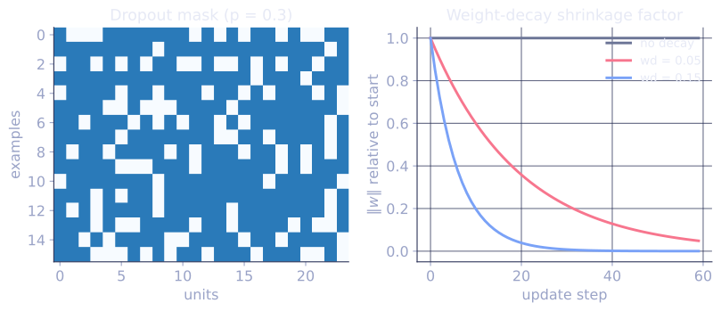
x_train = dropout(x, p=0.3, training=True, rng=rng)
x_eval  = dropout(x, p=0.3, training=False, rng=rng)
print(f"during training: zeros = {(x_train == 0).mean():.2f}, sum = {x_train.sum():.1f}")
print(f"during inference: identical to input? {np.allclose(x_eval, x)}")

# Weight decay shrinks parameters toward zero each step
def sgd_step(w, grad, lr=0.01, wd=0.0):
    return (1 - lr * wd) * w - lr * grad

w = np.array([3.0, -2.0, 1.5])
grad_zero = np.zeros_like(w)
# With wd=0 and zero gradient, weight is unchanged; with wd, it shrinks geometrically.
w_no_wd = w.copy(); w_wd = w.copy()
for _ in range(100):
    w_no_wd = sgd_step(w_no_wd, grad_zero, lr=0.01, wd=0.0)
    w_wd    = sgd_step(w_wd, grad_zero, lr=0.01, wd=0.1)
print(f"\nafter 100 zero-gradient steps:")
print(f"  no weight decay: {w_no_wd}")
print(f"  wd=0.1:          {w_wd.round(4)}  (decayed by (1 - 0.001)^100 = {(1 - 0.001)**100:.4f})")

# Both together: dropout + weight decay on a toy regression in the
# high-noise / modest-signal regime (50 features, noise variance 4x the
# per-coordinate signal variance) where unregularized OLS overfits the
# training noise and shrinkage / dropout each cut validation MSE.
N, d = 80, 50
X = rng.normal(size=(N, d))
y = X @ (0.5 * rng.normal(size=d)) + 2.0 * rng.normal(size=N)

def fit(X, y, p_drop, wd, n_iter=4000, lr=0.02, rng=rng):
    w = np.zeros(X.shape[1])
    for _ in range(n_iter):
        x_drop = dropout(X, p=p_drop, training=True, rng=rng)
        grad = x_drop.T @ (x_drop @ w - y) / len(X)
        w = (1 - lr * wd) * w - lr * grad
    return w

# Held-out evaluation
val_idx = rng.permutation(N)[:30]
train_idx = np.setdiff1d(np.arange(N), val_idx)
w_plain  = fit(X[train_idx], y[train_idx], p_drop=0.0, wd=0.0)
w_drop   = fit(X[train_idx], y[train_idx], p_drop=0.1, wd=0.0)
w_wd     = fit(X[train_idx], y[train_idx], p_drop=0.0, wd=0.05)
w_both   = fit(X[train_idx], y[train_idx], p_drop=0.1, wd=0.05)

for name, w in [("plain", w_plain), ("dropout", w_drop), ("wd", w_wd), ("both", w_both)]:
    val_mse = np.mean((X[val_idx] @ w - y[val_idx])**2)
    print(f"{name:>8}: val MSE = {val_mse:.4f}, ||w|| = {np.linalg.norm(w):.3f}")

Dropout zeros a fraction of features during training, weight decay shrinks parameters geometrically, and in this noisy regression each one (or both together) reduces validation MSE relative to plain unregularized training.

Exercises

Exercise 1. A dropout layer uses drop probability $p = 0.2$ with the inverse-keep-probability rescaling: a kept activation is multiplied by $1/(1-p)$, a dropped one by $0$. Show that the expected value of a single activation $a$ under the random mask equals $a$ itself, so training-time dropout is unbiased.

Exercise 2. Weight decay updates a parameter with zero gradient as $\theta_{t+1} = (1 - \eta\lambda)\,\theta_t$. Show that after $T$ steps the parameter has shrunk geometrically, and compute the factor for $\eta = 0.01$, $\lambda = 0.1$, $T = 200$.

Exercise 3 (code). L2 weight decay is MAP estimation with a Gaussian prior, which on a linear regression is ridge regression. Verify this equivalence: run the weight-decay SGD update to convergence on a small regression and check that it lands on the closed-form ridge solution $\hat\theta = (X^\top X + \alpha I)^{-1} X^\top y$.

import numpy as np

rng = np.random.default_rng(0)

N, d = 200, 5
X = rng.normal(size=(N, d))
theta_true = rng.normal(size=d)
y = X @ theta_true + 0.1 * rng.normal(size=N)

# Weight decay corresponds to a penalty (lambda_pen / 2) * ||theta||^2 in
# the loss. The full-batch MSE gradient is (1/N) X^T (X theta - y); the
# decay adds lambda_pen * theta, so the ridge penalty is alpha = N * lambda_pen.
lr, lambda_pen, n_iter = 0.05, 0.2, 50_000
alpha = N * lambda_pen

theta = np.zeros(d)
for _ in range(n_iter):
    grad = X.T @ (X @ theta - y) / N
    theta = (1 - lr * lambda_pen) * theta - lr * grad

theta_ridge = np.linalg.solve(X.T @ X + alpha * np.eye(d), X.T @ y)

assert np.allclose(theta, theta_ridge, atol=1e-4)
print("SGD-with-decay:", theta.round(4))
print("closed-form ridge:", theta_ridge.round(4))

The next lesson chooses the right optimizer for the resulting regularized objective.