Optimizers for deep learning

A3 covered the optimizer family in general; this lesson focuses on the deep-learning specifics: AdamW as the default for Transformers, the learning-rate schedule that makes the difference between training and failing to train, and the batch size that decides everything else. The math is the same as A3; the practice is where the choices matter.

SGD with momentum

The classic optimizer for vision:

With $\beta = 0.9$ and a learning-rate schedule, SGD with momentum trains ResNets to state-of-the-art accuracy. It is the default for image classification.

Strengths: robust generalization, well-understood, no per-parameter state beyond momentum.

Weaknesses: needs careful learning-rate tuning, struggles with very unequal gradient scales (which Transformers have).

Adam and AdamW

Adam from A3 maintains per-parameter first and second moments[1]. AdamW fixes Adam's coupling between weight decay and adaptive rescaling:

• Plain Adam adds $\lambda \theta$ to the gradient before computing $m$, $v$, and the update. The L2 term gets divided by $\sqrt{\hat v}$, so high-curvature directions get less decay than flat ones.
• AdamW applies weight decay after the adaptive step, decoupled from the gradient:

A concrete contrast makes the coupling visible. Take two coordinates at $\theta = 1$ with weight decay $\lambda = 0.1$, one in a flat direction (curvature 1, so gradient $g \approx 1$) and one in a steep direction (curvature 100, so $g \approx 100$). Adam divides the decay term by $\sqrt{\hat v} \approx |g|$:

• Flat direction: effective decay $\lambda / |g| = 0.1 / 1 = 0.1$.
• Steep direction: effective decay $0.1 / 100 = 0.001$.

The flat coordinate gets decayed $100\times$ harder than the steep one, the ratio of their curvatures, even though both were assigned the same $\lambda$. AdamW removes the division: the decay is $\lambda\theta = 0.1$ in both directions, identical regardless of curvature. That is the entire fix, and it is why AdamW consistently outperforms Adam at the same weight-decay value and is the default for Transformer training.

Learning-rate schedules

The single most important hyperparameter after the learning rate itself is its schedule over training:

• Step decay: multiply by 0.1 every $N$ epochs. Classic for CNNs.
• Cosine decay: smoothly anneal from initial LR to a tiny value via $\eta_t = \eta_0\,\tfrac{1}{2}(1 + \cos(\pi t / T))$. Standard for Transformers.
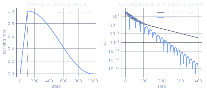
• Warmup + cosine: linearly increase the LR from 0 to $\eta_0$ over the first 1-5% of training, then cosine decay to zero. The standard for any Adam-trained Transformer.

Why warmup: Adam's running statistics $\hat m, \hat v$ are unreliable in the first few hundred steps (large bias-correction factors), so taking full-size steps then leads to instability[2]. Linear warmup lets the statistics stabilize before the steps grow.

Why cosine decay: late-training small steps are needed to land in a good local minimum without bouncing. Constant LR plus early stopping is a reasonable alternative.

Batch size

The batch size couples to every other hyperparameter:

• Larger batches give lower-variance gradients, so a bigger step is safe. Standard rule: linear scaling of LR with batch size up to some threshold; sqrt scaling for Adam at very large batches.
• **Effective batch size = batch * gradient-accumulation-steps **. Gradient accumulation simulates large batches when memory is tight.
• Critical batch size: a problem-dependent ceiling above which larger batches don't proportionally reduce the number of steps needed. Empirically in the thousands for vision, tens of thousands for language.

Gradient clipping

Long-tailed gradient distributions (especially in RNNs and Transformers early in training) can produce occasional enormous gradients that wreck the optimizer state. Gradient clipping:

caps the global gradient norm at $c$ (typically 1.0). Standard in language model training, almost free to apply.

A modern default recipe

For a fresh Transformer:

• Optimizer: AdamW, $\beta_1 = 0.9$, $\beta_2 = 0.95$, $\varepsilon = 10^{-8}$.
• Weight decay: 0.1, applied only to matrix parameters (not biases or norms).
• Learning rate: linear warmup for 1-5% of steps, then cosine decay to zero.
• Peak LR: $2 \times 10^{-4}$ to $10^{-3}$, scaled by batch size.
• Gradient clipping at norm 1.0.

For a fresh CNN:

• Optimizer: SGD with Nesterov momentum 0.9.
• Weight decay: $10^{-4}$ to $5 \times 10^{-4}$.
• Cosine LR decay from $\sim 0.1$ to 0.
• No gradient clipping needed.

Surprisingly little tuning is needed for either recipe to work; the defaults are a strong starting point.

Check it on arrays

import numpy as np

rng = np.random.default_rng(0)

# Quadratic objective with badly scaled coordinates (the AdamW use case)
H_diag = np.array([1.0, 100.0, 10.0, 1.0])
def loss(theta): return 0.5 * np.sum(H_diag * theta**2)
def grad(theta): return H_diag * theta

def sgd_momentum(theta0, lr, n_steps, beta=0.9):
    theta = theta0.copy(); v = np.zeros_like(theta)
    losses = []
    for _ in range(n_steps):
        v = beta * v + grad(theta)
        theta = theta - lr * v
        losses.append(loss(theta))
    return losses

def adamw(theta0, lr, n_steps, b1=0.9, b2=0.95, wd=0.01, eps=1e-8):
    theta = theta0.copy(); m = np.zeros_like(theta); v = np.zeros_like(theta)
    losses = []
    for t in range(1, n_steps + 1):
        g = grad(theta)
        m = b1 * m + (1 - b1) * g
        v = b2 * v + (1 - b2) * g * g
        mhat = m / (1 - b1**t); vhat = v / (1 - b2**t)
        theta = theta - lr * (mhat / (np.sqrt(vhat) + eps) + wd * theta)
        losses.append(loss(theta))
    return losses

theta0 = np.array([1.0, 1.0, 1.0, 1.0])
sgd_losses  = sgd_momentum(theta0, lr=0.01, n_steps=300)
adam_losses = adamw(theta0, lr=0.1, n_steps=300, wd=0.0)

print(f"loss after 50 steps:  SGD={sgd_losses[49]:.3e},  AdamW={adam_losses[49]:.3e}")
print(f"loss after 300 steps: SGD={sgd_losses[299]:.3e}, AdamW={adam_losses[299]:.3e}")

# Cosine schedule with warmup
def cosine_warmup(t, warmup, total, base_lr):
    if t < warmup:
        return base_lr * t / warmup
    progress = (t - warmup) / (total - warmup)
    return base_lr * 0.5 * (1 + np.cos(np.pi * progress))

base_lr = 1e-3; warmup = 100; total = 1000
schedule = [cosine_warmup(t, warmup, total, base_lr) for t in range(total)]
print(f"\nschedule values: t=0 -> {schedule[0]:.2e}, t={warmup} -> {schedule[warmup]:.2e}, t={total-1} -> {schedule[-1]:.2e}")

AdamW closes the ill-conditioned quadratic far faster than SGD with momentum because it rescales per coordinate; the warmup-cosine schedule starts at zero, peaks at warmup, and decays to zero.

Exercises

Exercise 1. Take one AdamW step by hand on a single coordinate. With $\theta_0 = 1$, gradient $g = 2$, $\beta_1 = 0.9$, $\beta_2 = 0.999$, $\eta = 0.1$, $\lambda = 0.1$, $\varepsilon = 0$, and zero-initialized moments, compute $\theta_1$.

Exercise 2. Show why plain Adam couples weight decay to curvature. For two coordinates with the same decay $\lambda$ but second-moment estimates $\hat v_a = 1$ and $\hat v_b = 100$, compute the effective decay each receives when the $\lambda\theta$ term is folded into the gradient (so it passes through the $1/\sqrt{\hat v}$ rescaling).

Exercise 3 (code). Implement a step-decay schedule (multiply the base LR by $0.1$ every $N$ epochs) and assert it produces the expected piecewise-constant values. Then confirm the warmup-cosine schedule from the lesson is continuous at the warmup boundary.

import numpy as np

def step_decay(epoch, base_lr=0.1, drop=0.1, every=30):
    return base_lr * drop ** (epoch // every)

assert np.isclose(step_decay(0), 0.1)
assert np.isclose(step_decay(29), 0.1)
assert np.isclose(step_decay(30), 0.01)
assert np.isclose(step_decay(60), 0.001)

def cosine_warmup(t, warmup, total, base_lr):
    if t < warmup:
        return base_lr * t / warmup
    progress = (t - warmup) / (total - warmup)
    return base_lr * 0.5 * (1 + np.cos(np.pi * progress))

base_lr, warmup, total = 1e-3, 100, 1000
# At the boundary the warmup ramp reaches base_lr and cosine starts at base_lr
left = cosine_warmup(warmup - 1, warmup, total, base_lr)
peak = cosine_warmup(warmup, warmup, total, base_lr)
assert np.isclose(peak, base_lr)
assert abs(peak - left) < base_lr / warmup + 1e-12   # continuous to one ramp step
print("step decay and warmup-cosine schedules verified")

This closes the D1 core-building-blocks track. The next subsection (D2) applies these foundations to image data with convolutional networks.

References

- [1]Kingma, D. P., & Ba, J. (2015). "Adam: a method for stochastic optimization". ICLR. arXiv:1412.6980. The adaptive optimizer with per-parameter first and second moment estimates.↩
- [2]Goodfellow, I., Bengio, Y., & Courville, A. (2016). Deep Learning, §8.5 (Algorithms with Adaptive Learning Rates). MIT Press. Adaptive-rate optimizers and the practical tuning of their schedules.↩